
Abstract
Version 1.2 of the software system, termed Crystallography and NMR system (CNS), for crystallographic and NMR structure determination has been released. Since its first release, the goals of CNS have been (i) to create a flexible computational framework for exploration of new approaches to structure determination, (ii) to provide tools for structure solution of difficult or large structures, (iii) to develop models for analyzing structural and dynamical properties of macromolecules and (iv) to integrate all sources of information into all stages of the structure determination process. Version 1.2 includes an improved model for the treatment of disordered solvent for crystallographic refinement that employs a combined grid search and least-squares optimization of the bulk solvent model parameters. The method is more robust than previous implementations, especially at lower resolution, generally resulting in lower R values. Other advances include the ability to apply thermal factor sharpening to electron density maps. Consistent with the modular design of CNS, these additions and changes were implemented in the high-level computing language of CNS.
Introduction
The program CNS was the first advanced software system in structural biology that made use of a modular, multilevel approach to computing, utilizing a high-level symbolic structure-determination language1. Since its first dissemination in 1998, CNS has become one of the most widely used systems to determine structures based on X-ray diffraction or nuclear magnetic resonance data or both. Its key advantages are the flexibility and generality of the system, allowing 'computational experimentation' with new algorithms or applications to different types of experimental data without tedious software development.
In CNS, many algorithms were moved from the source code into this symbolic language. The high-level CNS computing language allows definition of symbolic target functions, data structures, procedures and modules. The compiled CNS program, written in Fortran77, acts as an interpreter for the high-level CNS language and includes hard-wired functions for the efficient processing of computing-intensive tasks. Methods and algorithms are therefore more clearly defined and easier to adapt to new and challenging problems. The result is a multilevel system that provides maximum flexibility to the user. The CNS language provides a common framework for nearly all the computational procedures required for structure determination. A comprehensive set of crystallographic procedures for phasing, density modification and refinement has been implemented in this language. The CNS language permits the design and execution of nearly any numerical task in structure determination, using a minimal set of 'hard-wired' functions and routines. Task files consist of CNS language statements and module invocations. The task files, which can also be accessed, modified or viewed through an HTML graphical interface, are available to carry out these procedures.
Most operations within a structure-determination algorithm are defined through modules and task files. This allows the development of new algorithms and for existing algorithms to be precisely defined and easily modified without the need for source code modifications. This hierarchical structure of CNS allows extensive testing at each level. For example, once the source code and CNS basic commands have been tested, testing of the modules and task files can be performed. A test suite consisting of hundreds of test cases is available to detect and correct programming errors. This testing scheme makes CNS highly reliable. It also makes it easier to modify the program and add new features.
The source codes of CNS and its predecessor X-PLOR (see ref. 2) are available, allowing users to easily interface their algorithms with these programs. Examples of such interfaces include tools developed for NMR structure determination3, the protein–protein docking method HADDOCK based on biochemical and/or biophysical information4, the ARIA method for automated NOE assignment and NMR structure calculation5, incorporation of electrostatics and continuum dielectric methods in refinement6, a database of interatomic distance probabilities7, time-averaged molecular dynamics refinement against X-ray diffraction data8 and molecular dynamics in refinement against fiber diffraction data9.
The major new features of version 1.2 of CNS include an improved bulk solvent model for crystallographic refinement and the ability to manipulate electron density maps by thermal factor sharpening. These and most other changes in the system were restricted to the high-level task and module files (Supplementary Note online).
Bulk solvent modeling in X-ray crystallography
The correct modeling of the barrier between the bulk solvent in the crystal lattice and the protein itself is an important part of macromolecular structure refinement. The structure factor Fcalc of a macromolecular crystal structure is expressed in CNS as

where the structure factor Fmacro is obtained from the atomic model of the macromolecule, Fbound is computed from all bound water molecules, Fbulk is obtained from an appropriate model for disordered solvent, h→ is a column vector with the Miller indices of a Bragg reflection, 't' denotes the transpose of it (i.e., a row vector) and the symmetric second rank tensor U describes overall mean-square displacements of the crystal lattice (dimensionless anisotropic mean-square displacements (ADPs)). The isotropic component of the ADPs is usually separated from U and applied directly to Fmacro, Fbound and Fbulk. To do this, the U tensor is converted into Cartesian coordinate space Ucart (see ref. 10). One-third of its trace (i.e., Ucart[11] + Ucart[22] + Ucart[33])/3) is the isotropic thermal factor contribution.
To compute Fbulk, a mask is created to distinguish between macromolecular and solvent regions. This problem is closely related to the computation of accessible and molecular surface areas11. A three-dimensional map mask is defined on a grid that covers an asymmetric unit of the crystal. The values of mask are restricted to 0 and 1. The grid size is chosen to be small enough to avoid Fourier series truncation errors. By trial and error, we set the grid size to one-third of the high-resolution limit with the additional condition that the grid must be in the range between 0.57 and 0.9 Å.
All grid points of mask are initially set to 1. Grid points of mask within a distance of ri around any atom i of the atomic model and its symmetry mates are then set to 0. The atomic model includes the macromolecule and any bound water molecules or ligands. ri is defined as the sum of the van der Waals radius rvdw of atom i and the probe radius rprobe. The van der Waals radius is defined as half the distance at which the Lennard-Jones potential energy function reaches its minimum.
All grid points of mask marked 0 are tested to see if they fall within a distance rshrink from a grid point set to 1. If this is the case, the tested grid point is set to 1. This procedure effectively 'shrinks' the accessible surface area. The resulting boundary between solvent and macromolecule is a combination of contact and reentrant surface areas12. The grid points of mask marked 1 comprise the solvent regions, whereas those marked 0 are associated with the atomic model and its symmetry mates.
The widely used 'flat' solvent model assumes that solvent regions outside the molecular surface show relatively little variation in density as compared to the macromolecule13. The structure factor of the solvent Fbulk is then simply computed by Fourier transformation of mask. To blur the sharp boundary between macromolecule and solvent as imposed by the mask, resolution-dependent scaling in reciprocal space is applied using an isotropic 'thermal' factor Bsol:

where FT denotes the three-dimensional Fourier transformation, and ksol is a scale factor that defines the mean electron density in the solvent region. Thus, for a well-behaved solvent model, ksol should be close to 0.3 e Å−3 and Bsol reasonably close (within a factor 2) to the average thermal factor of the macromolecular model.
The optimum solvent model is obtained by minimizing the expression

where Fobs is the observed structure factor. Due to the implementation of fundamental features in the CNS source code, the optimization is broken up into optimization of isotropic and anisotropic parameters (Table 1). The bulk solvent procedure in the earlier versions of CNS often resulted in numerical instabilities for the refinement of the solvent parameters ksol and Bsol, for structures determined at low to moderate resolution (i.e., lower than 3 Å resolution). The procedure was therefore modified by introduction of a grid search for ksol. It was found to be sufficient to perform the grid search only for ksol, while letting Bsol and the other scale factors being determined by least-squares optimization for each selected value of ksol (Table 1). Others have found a similar solution to this problem involving a grid search of both ksol and Bsol (see ref. 14). On a rare occasion, the CNS 1.2 procedure produces a non-converging solution for a particular value of ksol, which is then excluded by choosing the minimum R-value solution for the entire search.
It should be noted that proper implementation of the overall anisotropic thermal factor refinement is complicated by restrictions imposed by crystallographic symmetry on the individual components of the thermal factor tensor10. To simplify the calculations, the diffraction data are temporarily expanded to space group P1, the overall anisotropic thermal factor refinement is performed in P1, followed by reduction to the particular space group. This procedure ensures the proper symmetry restrictions on the thermal factor tensor while the computational overhead in P1 is not of particular concern on modern computing platforms.
For refinements at medium to high resolution (up to around 3 Å resolution), Rprobe = Rshrink = 1 is the optimum choice15. However, for the refinement of the ATPase p97/VCP at 4.5 Å resolution, it was necessary at the early stages of the refinement to adjust Rprobe and Rshrink for computation of the bulk solvent mask to obtain optimum R and Rfree values16,17. Initially, optimization showed that different values for each of the Rprobe and Rshrink parameters could produce a slightly lower Rfree. However, in the final refinement stages, equal values of Rprobe and Rshrink produced optimum results. Thus, in CNS 1.2, both parameters are changed simultaneously with Rshrink = Rprobe. Furthermore, both values tend to approach the value of 1 as the atomic model is being completed and improved.
This entire procedure was implemented with new modules ('scale_and_solvent' and 'scale_and_solvent_grid_search') and suitably modified task files without any source code modification. Extensive testing indicated that the CNS 1.2 bulk solvent model is robust for structures solved at both high and low resolution. The new solvent model may require significantly more computing time in the start-up phase of refinement tasks compared to the previous version. However, compared to the overall computing time for refinement, this additional time is usually insignificant. The new method often yields lower R values than the previous version of CNS.
Thermal factor sharpening of electron density maps
Thermal ('B')-factor sharpening is a useful tool for enhancement of low-resolution maps16,17,18,19. Thermal factor sharpening entails the use of a negative Bsharp value in a resolution-dependent weighting scheme applied to a particular electron density map:

where Fmap is the structure factor of the particular electron density map, Fsharpened_map is the structure factor of the sharpened map, θ is the reflecting angle and λ is the wavelength of the X-ray radiation. Applying a negative Bsharp value effectively up-weights higher resolution terms. The result of this weighting scheme is increased detail for higher resolution features such as side-chain conformations. However, the cost of the increased detail can be increased noise throughout the electron density map. Sometimes, the noise can coincide with regions of backbone or side-chain electron density, producing potential artifacts. Thus, thermal factor sharpening is a density-modification technique that is only as good as the diffraction data and phases that are available, and therefore, the original unweighted electron density maps should always be considered. Furthermore, little improvement is observed on electron density maps that are computed with phases derived solely from molecular replacement, so experimental phase information appears to be important to get the most benefit from thermal factor sharpening16.
Thermal factor sharpening can be viewed as a simple weighting function applied to the observed amplitudes and consequently the electron density maps by virtue of relative scaling between atomic model and observed amplitudes. In the case of the crystal structure of the ATPase p97/VCP, the Bsharp value that produced the most useful electron density map coincided with the smallest absolute value of Bsharp that results in a Wilson plot that is positive in all resolution bins19. The new task file 'bsharp.inp' implements this approach for determining Bsharp. However, it remains to be seen if this empirical rule applies to the general case. Thermal factor sharpening can also be viewed as a pseudo Wilson scaling of the diffraction data, so another reasonable choice for Bsharp would be to set it to the negative Wilson B value of the diffraction data.
The implementation in version 1.2 of CNS applies equation (4) at the step just before application of the fast Fourier transformation to compute the actual three-dimensional map. In other words, the Fourier coefficients for the particular electron density map are computed and then equation (4) is applied to them. Thus, this procedure works for any type of electron density map based on experimental or model phases and with any type of weighting or phase-combination scheme. The only required modifications involved changes of the CNS task and module files related to electron density map calculations. No changes in the FORTRAN source code were required. The thermal factor sharpening feature does not impose any particular additional computational time compared to the previous version of CNS. One could envision a generalization to anisotropic thermal factor sharpening that could be particularly useful for highly anisotropic crystals.
The procedure contains two examples of how the new features of CNS can be used. The first example is for crystallographic refinement and the second example is for computing an electron density map.
Materials
Equipment
-
A computer with access to the Internet and a web browser. Implementations for some of the most common operating systems are available, including Linux and Mac OS X.
-
Data All CNS data formats are text files. For coordinates, the format of the Protein Data Bank (PDB)20 is supported. For diffraction data, conversion programs are available in CNS and the CCP4 suite21 to import files generated by commonly used data reduction programs.
-
Programs The CNS website http://cns-online.org contains all task files ('Input Files'), parameter and library files for the program ('Libraries'), the module files ('Modules'), information about specific hardware implementations ('Installation'), a syntax manual ('Syntax Manual') and a tutorial for the most common tasks ('Tutorial'). This website can also be used to modify the task files and assign default values to certain parameters, such as the unit cell dimensions and space group symmetry. The website provides information on how to obtain the CNS program. The user performs the calculations on local computers using task files downloaded or modified by the CNS website. To execute a task file on a local computer, it is advisable to create a directory that contains all required input files. In a UNIX environment, CNS is executed by the following command:
CNS < input_file > output_file
Procedure
-
1
The starting coordinate file must be in the PDB format. Convert the diffraction data file to the CNS format.
-
2
Go to the CNS website's 'Input Files' section.
-
3
Set the default parameters (space group, cell dimensions and optionally, anomalous form factors) by going to the 'Set' menu, and then click on 'Start editing files'.
-
4
If the diffraction data file already contains a test set for cross-validation, skip this step. Otherwise, select the task file 'make_cv.inp' in the 'Refinement' section. Enter any changes that may be required. Save the file to a local computer and execute CNS. The task file creates a new diffraction data file that contains the test set information in addition to the observed data.
-
5
If you would like to continue with the general crystallographic refinement task file ('refine.inp') or compute an electron density map, follow option A or B respectively.
-
A
General crystallographic refinement
-
i
Select the task file 'refine.inp' in the 'Refinement' section and enter information that is required, such as the name of the coordinate file, the diffraction data file with test set (e.g., generated by the previous step) or the name of the output coordinate file. If the structure contains ligands or other non-standard residues, the 'generate.inp' task file in the 'General' section has to be run first to generate a 'molecular topology' file. If the protein contains cis peptide bonds, except for proline, a special parameter file needs to be generated by the task file 'cis_peptide.inp' in the 'General' section and the resulting parameter file read in all subsequent refinement tasks.
-
ii
Read additional restraints, such as non-crystallographic symmetry restraints or constraints.
-
iii
Change options and parameters of the 'refine.inp' task file as required. The default values should be reasonable for most cases. The following is a screenshot of a section of the task file relevant to bulk solvent modeling (Fig. 1).
Figure 1 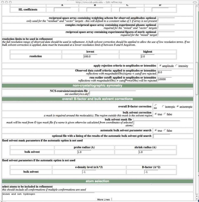
A screenshot of a section of the task file relevant to bulk solvent modeling.
-
iv
Save the file to your local computer and execute CNS. Examine the output file for errors. Usually, it is sufficient to go to the bottom of the output file and make sure that it is saved normally without an abort message.
-
v
The coordinate file that is generated by 'refine.inp' contains useful information at the top of the file (see ANTICIPATED RESULTS). The resulting coordinate file can be viewed or further manipulated with any molecular graphics program that supports the PDB format.
-
i
-
B
Computation of an electron density map
-
i
Select the 'model_map' task file in the 'Refinement' section. Change options and parameters of the task file, as required. The default values should be reasonable for most cases. The following is a screenshot of a section of the task file (Fig. 2). Note the line that specifies the thermal ('B') factor sharpening.
Figure 2 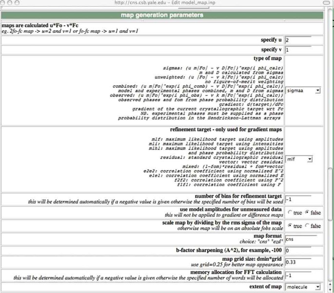
A screenshot of a section of the task file for computation of an electron density map.
-
ii
Save the file to a local computer and execute CNS. Examine the output file for errors. Usually, it is sufficient to go to the bottom of the output file and make sure that it is saved normally without an abort message.
-
i
-
A


Anticipated results
Figure 3 shows the top of the refined PDB file produced by the task file 'refine.inp'.

The top of the refined PDB file produced by the task file 'refine.inp'.
Examine the reduction in R values and the values of the bulk solvent model. A significant increase of the free R value indicates problems with the model. The Bsol parameter should be within a factor of 3 of the average B value of the atomic model, and the ksol parameter should be reasonably close to the expected value of water electron density (∼0.3 e Å−3). The coordinate file also contains information about the local geometry of the refined model (average deviation of bond lengths and bond angles from ideal values) and the variation of thermal factors for atoms connected through one or two bonds.
A thermal factor sharpened map should always be compared with the original map that was computed without thermal factor sharpening, as artifacts can be introduced by thermal factor sharpening.
Note: Supplementary information is available via the HTML version of this article.
References
Brunger, A.T. et al. Crystallography & NMR system: a new software suite for macromolecular structure determination. Acta Crystallogr. 54 (Part 5): 905–921 (1998).
Brunger, A.T. X-PLOR, version 3.1. A System for X-ray Crystallography and NMR (Yale University Press, New Haven, Connecticut, USA, 1992).
Schwieters, C.D., Kuszewski, J.J., Tjandra, N. & Clore, G.M. The Xplor-NIH NMR molecular structure determination package. J. Magn. Reson. 160, 65–73 (2003).
Dominguez, C., Boelens, R. & Bonvin, A.M. HADDOCK: a protein–protein docking approach based on biochemical or biophysical information. J. Am. Chem. Soc. 125, 1731–1737 (2003).
Linge, J.P., Habeck, M., Rieping, W. & Nilges, M. ARIA: automated NOE assignment and NMR structure calculation. Bioinformatics (Oxford, England) 19, 315–316 (2003).
Moulinier, L., Case, D.A. & Simonson, T. Reintroducing electrostatics into protein X-ray structure refinement: bulk solvent treated as a dielectric continuum. Acta Crystallogr. 59, 2094–2103 (2003).
Wall, M.E., Subramaniam, S. & Phillips, G.N. Jr. Protein structure determination using a database of interatomic distance probabilities. Protein Sci. 8, 2720–2727 (1999).
Clarage, J.B. & Phillips, G.N. Jr. Cross-validation tests of time-averaged molecular dynamics refinements for determination of protein structures by X-ray crystallography. Acta Crystallogr. 50, 24–36 (1994).
Wang, H. & Stubbs, G. Molecular dynamics in refinement against fiber diffraction data. Acta Crystallogr. A 49, 504–513 (1993).
Grosse-Kunstleve, R. & Adams, P. On the handling of atomic anisotropic displacement parameters. J. Appl. Crystallogr. 35, 477–480 (2002).
Lee, B. & Richards, F.M. The interpretation of protein structures: estimation of static accessibility. J. Mol. Biol. 55, 379–400 (1971).
Richards, F.M. Calculation of molecular volumes and areas for structures of known geometry. Methods Enzymol. 115, 440–464 (1985).
Phillips, S.E. Structure and refinement of oxymyoglobin at 1.6 Å resolution. J. Mol. Biol. 142, 531–554 (1980).
Afonine, P.V., Grosse-Kunstleve, R.W. & Adams, P.D. A robust bulk-solvent correction and anisotropic scaling procedure. Acta Crystallogr. 61, 850–855 (2005).
Jiang, J.S. & Brunger, A.T. Protein hydration observed by X-ray diffraction. Solvation properties of penicillopepsin and neuraminidase crystal structures. J. Mol. Biol. 243, 100–115 (1994).
DeLaBarre, B. & Brunger, A.T. Complete structure of p97/valosin-containing protein reveals communication between nucleotide domains. Nat. Struct. Biol. 10, 856–863 (2003).
DeLaBarre, B. & Brunger, A.T. Nucleotide dependent motion and mechanism of action of p97/VCP. J. Mol. Biol. 347, 437–452 (2005).
Bass, R.B., Strop, P., Barclay, M. & Rees, D.C. Crystal structure of Escherichia coli MscS, a voltage-modulated and mechanosensitive channel. Science 298, 1582–1587 (2002).
DeLaBarre, B. & Brunger, A.T. Considerations for the refinement of low-resolution crystal structures. Acta Crystallogr. 62, 923–932 (2006).
Westbrook, J.D. & Fitzgerald, P.M. The PDB format, mmCIF, and other data formats. Methods Biochem. Anal. 44, 161–179 (2003).
CCP. The CCP4 suite: programs for protein crystallography. Acta Crystallogr. 50, 760–763 (1994).
Acknowledgements
I am grateful to Paul Adams and Byron DeLaBarre for stimulating discussions.
Author information
Authors and Affiliations
Corresponding author
Supplementary information
Supplementary Note
List of Changes for Version 1.2 (PDF 74 kb)
Rights and permissions
About this article
Cite this article
Brunger, A. Version 1.2 of the Crystallography and NMR system. Nat Protoc 2, 2728–2733 (2007). https://doi.org/10.1038/nprot.2007.406
Published:
Issue Date:
DOI: https://doi.org/10.1038/nprot.2007.406
This article is cited by
-
Staphylococcus aureus sacculus mediates activities of M23 hydrolases
Nature Communications (2023)
-
Artificial intelligence for template-free protein structure prediction: a comprehensive review
Artificial Intelligence Review (2023)
-
Structural and biochemical characterizations of Thermus thermophilus HB8 transketolase producing a heptulose
Applied Microbiology and Biotechnology (2023)
-
Structural analysis of Red1 as a conserved scaffold of the RNA-targeting MTREC/PAXT complex
Nature Communications (2022)
-
Controlling oncogenic KRAS signaling pathways with a Palladium-responsive peptide
Communications Chemistry (2022)
Comments
By submitting a comment you agree to abide by our Terms and Community Guidelines. If you find something abusive or that does not comply with our terms or guidelines please flag it as inappropriate.
