
Abstract
In this paper, a family of the weighted polymer networks is introduced depending on the number of copies f and a weight factor r. The topological properties of weighted polymer networks can be completely analytically characterized in terms of the involved parameters and/or of the fractal dimension. Moreover, assuming that the walker, at each step, starting from its current node, moves to any of its neighbors with probability proportional to the weight of edge linking them, namely weight-dependent walk. Then, we calculate the average receiving time (ART) with weighted-dependent walks, which is the sum of mean first-passage times (MFPTs) for all nodes absorpt at the trap located at the central node as a recursive relation. The obtained remarkable results display that when \(\frac{1}{f+1} < r < 1\), the ART grows sublinearly with the network size; when \(r=\frac{1}{f+1}\), ART grows with increasing size N g as \({\mathrm{ln}}^{2}{N}_{g}\); when \(0 < r < \frac{1}{f+1}\), ART grows with increasing size N g as ln N g . In the treelike polymer networks, ART grows with linearly with the network size N g when r = 1. Thus, the weighted polymer networks are more efficient than treelike polymer networks in receiving information.
Introduction
Complex networks, as a powerful tool to describe and characterize the natural and man-made systems, have attracted considerable attention in many fields, such as mathematics, biology, life science and engineering disciplines1,2,3. Besides, as rapid developing discipline, polymer science has attracted much attention in the past few years, since it provides a powerful tool to study the macromolecules with various structures4. Flexible polymer structures are various, such as dendrimers5, mesh-like polymers6, 7, fractals8, 9, dendritic10, 11, regular hyperbranched structures12, 13, scale-free and small-world networks14, 15, and so on.
Weighted networks represent the natural framework to describe natural, social, and technological systems, in which the intensity of a relation or the traffic between elements is an important parameters16, 17. In general terms, weighted networks are extension of networks or graphs18, 19, in which each edge between nodes i and j is associated with a variable w ij , called the weight. Much attention has been paid to the study of weighted networks because most real networks, which include airport networks20, ecosystems21, the Internet networks22 and so on, often show weighted properties, so it is also meaningful to investigate the behavior on the weighted networks23. Motivated by complex networks and polymer structures, Zhang et al. defined a category of treelike polymer networks controlled by a parameter, which is built in an iterative way24, 25. Combining the weighted networks26 and polymer structures, a family of the weighted polymer networks is introduced depending on the number of copies f and a weight factor r.
In 2015, Dai et al. introduced comprehensively three kinds of walks: random walk, weigh-dependent walk and strength-dependent walk on the weighted networks27. On weighted networks, the walker will choose an edge according to its weight of the node connected by it, i.e. weight-dependent walk. A key quantity related to weighted networks is the mean first-passage time(MFPT), that is, the expected first time for the walker starting from a source node to a given target node. The average receiving time (ART) is the sum of mean first-passage times (MFPTs) for all nodes absorpt at the trap located at a given target node28,29,30,31.
In this paper, we define a family of weighted polymer networks controlled by two parameters, which is built in an iterative way. According to the construction, we study some structural properties of the weighted polymer networks, showing that (1) in the limit of large network order g, the average degree of weighted polymer networks tends to 2; (2) when 0 < r < 1, their average node strength goes to zero as g increases; (3) their node strength distribution follows a power-law distribution; (4) the weighted polymer networks networks have small-world property: in the infinite network, the average weighted shortest path (AWSP) tends to be a constant value which depends on two parameters f, r. However, the average shortest path (ASP) increases logarithmically with the network size. Then, by applying recursive relations of weighted polymer networks, we calculate the average receiving time (ART) with weighted-dependent walks, which is the sum of mean first-passage times (MFPTs) for all nodes absorpt at the trap located at the central node. So we derive exactly the ART formula, which displays that in large networks, the leading behaviors of ART for the weighted polymer networks follow distinct scalings, with the trapping efficiency associated with the network size N g , the number of copies f and a weight factor r.
This paper is organized as follow. Based on weighted networks26 and polymer structures, a family of the weighted polymer networks is introduced depending on the number of copies f and a weight factor r in the next section. In Section 3, some a priori prescribed topology is described in terms of average degree, average node strength, node strength distribution, and the average weighted shortest path, depending on the two main parameters: the number of copies f and the weight factor r. In Section 4, the average receiving time (ART) with weighted-dependent walk is obtained by recursive formulas for F 1(g) and T tot (g). In the last section, we draw some conclusions that (1) the topology of weighted polymer networks can be completely analytically characterized in terms of the involved parameters and/or of the fractal dimension; (2) the weighted polymer networks are more efficient than treelike polymer networks in term of receiving information.
Weighted treelike networks
In this section, a family of weighted polymer networks are introduced. Intuited by polymer networks24, 25 and Weighted Fractal Networks (WFN for short)26, a family of weighted polymer networks are constructed in a deterministically iterative way.
Let r(0 < r < 1) be a positive real numbers, and f(f ≥ 1) be a positive integer. Denote by G g the weighted polymer networks after g iterations, and the following is the iterative algorithm to create weighted polymer networks:
-
(1)
For g = 0, G 0 consists of an isolated node, called the central node. For g = 1, f new nodes are generated connecting the central node to form G 1. Let G 1 be our base graph, composed by f + 1 nodes and f edges with unit weight. The f + 1 nodes in G 1 are all the attaching nodes, labeled by \(0,1,2,\cdots ,f\).
-
(2)
For g = 2, G 2 is obtained from G 1: Let \({G}_{1}^{\mathrm{(0)}},{G}_{1}^{\mathrm{(1)}},\cdots ,{G}_{1}^{(f)}\) be f + 1 replicas of G 1, whose weighted edges have been scaled by the weight factor r. For \(i=0,1,2,\cdots ,f\), let us denote by i′ the central node in \({G}_{1}^{(i)}\). Then merge the central node i′ in \({G}_{1}^{(i)}\) and Node i in G 1 into a single new node, still labelled by \(i(i=0,1,\cdots ,f)\). Figure 1 illustrates the iterative construction processes of a particular network from g = 1 to g = 3 for the case of f = 3.
Figure 1 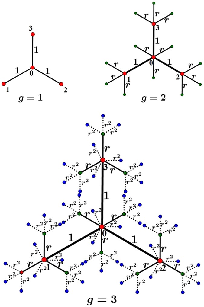
Iterative construction method for weighted polymer networks from g = 1 to g = 3 for the case of f = 3.
-
(3)
For g ≥ 1, G g is obtained from G g−1 (see Fig. 2): Let \({G}_{g-1}^{(0)},{G}_{g-1}^{(1)},\cdots ,{G}_{g-1}^{(f)}\) be f + 1 replicas of G g−1, whose weighted edges have been scaled by the weight factor r. For \(i=0,1,2,\cdots ,f\), let us denote by i′ the central node in \({G}_{g-1}^{(i)}\). Then merge the central node i′ in \({G}_{g-1}^{(i)}\) and Node i in G 1 into a single new node, still labelled by \(i(i=0,1,\cdots ,f)\). The weighted polymer networks is set up.
Figure 2 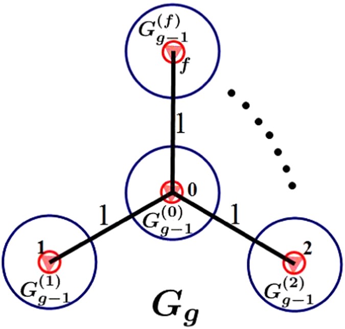
Construction method of weighted polymer networks. The open circles and triangles represent Node i′ of \({G}_{g-1}^{(i)}\) and i of \({G}_{1}(i=0,1,2,\cdots ,f)\), respectively.


The weighted polymer networks is one of type of WFN. According to Carletti and Righi26, WFN are scale-free, the exponent being the fractal dimension. WFN exhibit the “small-world” property (i.e. slow (logarithmic) increase of the average shortest path with the network size) and large average clustering coefficient. Thus, the fractal dimension of weighted polymer networks is completely characterized by two main parameters: the number of copies f ≥ 1 and the weight factor 0 < r < 1. We have that the fractal dimension of the weighted polymer networks is \({d}_{fract}=-\,\frac{\mathrm{log}(f+1)}{\mathrm{log}\,r}\).
According to the construction approach, it is easy to derive that at each iterative step g i (g i ≥ 1), the number of newly generated nodes is \(L({g}_{i})=f{(f+1)}^{{g}_{i}-1}\). Then the total number of nodes at each generation g is
and the total number of edges in G g is E g = N g − 1 = (f + 1)g − 1.
Topological properties of weighted polymer networks
The aim of this section is to characterize the topology of weighted polymer networks, by analytically studying their properties such as the average degree, the average node strength, the node strength distribution, and the average weighted shortest path.
Average degree and average node strength
The degree of a node i in a network, that is, the number of connections or edges the node i has to other nodes, is denoted by deg(i). The average degree of the weighted polymer networks G g , denoted by ad(G g ), is defined as \(ad({G}_{g})=\frac{2{E}_{g}}{{N}_{g}}\) 32. Hence in the limit of large g, the average degree ad(G g ) is finite and it is asymptotically given by
In the weighted polymer networks G g , a weight w ij is assigned to the edge connecting the nodes i and j, and the strength of node i can be defined as
where the sum index j runs over the set ν(i) of neighbors of i. The strength of a node integrates the information concerning its connectivity and the weights of its links33, 34. Then using the recursive construction, we can explicitly compute the total node strength \({S}_{g}={\sum }_{i\in {G}_{g}}{s}_{i}\), and, provided \(r\ne \frac{1}{f+1}\), easily show that
Because r < 1, we trivially find that the average node strength goes to zero as g increases: \({S}_{g}/{N}_{g}=\frac{2f{r}^{g}}{fr+r-1}-\frac{2f}{(fr+r-1){(f+1)}^{g}}\to 0(g\to \infty )\).
Especially, let us observe that the same is true if \(r=\frac{1}{f+1}\); in this case, in fact S g = 2fg grows linearly with g, thus slower than N g .
Node strength distribution
Let n(s) denote the number of nodes in the weighted polymer networks G g that have strength s. Let s i (g i ) be the strength of any one of newly generated nodes i at each iterative step g i (g i > 0). Assume that node i entered the networks at generation g(g > 0), then s i (g) = r g−1. By construction, the strength of node i entered the networks at generation g i (0 < g i < g) is \({s}_{i}({g}_{i})={r}^{{g}_{i}-1}+f({r}^{g-1}+{r}^{g-2}+\cdots +{r}^{{g}_{i}})\). For g i = 0, the strength of the initial central node labeled by 0, equals to \({s}_{0}(0)=f({r}^{g-1}+{r}^{g-2}+\cdots +r+1)\). Using the property of iterative construction method, we can conclude:
For g = 100, n(s) versus s in the weighted polymer networks is on a log-log scale in Fig. 3. The slope of the weighted polymer networks G 100 with 8100 nodes, f = 7 and r = 1/4 is −1.4992, which differs by 0.0008 from its the negative of the fractal dimension \(-{d}_{frac}=\frac{\mathrm{log}\,8}{\mathrm{log}\,1\,/\,4}=-\,1.5000\). The slope of the weighted polymer networks G 100 with 9100 nodes, f = 8 and r = 1/8 is −1.0565, which differs by 0.0001 from its the negative of the fractal dimension \(-{d}_{frac}=\frac{\mathrm{log}\,9}{\mathrm{log}\,1\,/\,8}=-\,1.0566\). The slope of the weighted polymer networks G 100 with 31100 nodes, f = 30 and r = 1/2 is −4.9339, which differs by 0.0203 from its the negative of the fractal dimension \(-{d}_{frac}=\frac{\mathrm{log}\,31}{\mathrm{log}\,1\,/\,2}=-\,4.9542\). The slope of the weighted polymer networks G 100 with 4100 nodes, f = 3 and r = 1/30 is −0.4077, which differs by −0.0001 from its the negative of the fractal dimension \(-{d}_{frac}=\frac{\mathrm{log}\,4}{\mathrm{log}\,1\,/\,30}=-\,0.4076\). The results show that for different weight factor r and different copy number f, every line slope of log n(s) versus log s is nearly equal to the negative of the fractal dimension \(-{d}_{fract}=\frac{\mathrm{log}(f+1)}{\mathrm{log}\,r}(0 < r < 1)\). This implies that n(s) are distributed according to a power law with exponent \({d}_{fract}=-\frac{\mathrm{log}(f+1)}{\mathrm{log}\,r}\). And therefore, for large g, n(s) can be obtained as
where c is constant. Thus, n(s) also follows a power-law distribution.

The log-log plot of n(s) versus s for different weight factor r and different copy number f.
Average weighted shortest path
By definition the average weighted shortest path(AWSP) of the weighted networks G g 35 is given by
where
d ij (g) being the weighted shortest path linking nodes i and j in G g .
The modular recursive construction of G g allows us to calculate the exact value of S tot (g). At step g + 1, we incise G g into f + 1 branches, which we label as \({G}_{g}^{(i)}(i=0,1,\cdots ,f)\). Each branch \({G}_{g}^{(i)}(i=0,1,\cdots ,f)\) is a copy of G g and has the same structure as G g , while their edge weights have been scaled by a weight factor r. The central nodes i′ of \({G}_{g}^{(i)}(i=1,\cdots ,f)\) are all connected to central node 0′ of \({G}_{g}^{(0)}\) by f edges with unit weight. Thus, the total of shortest distances S tot (g) satisfies the following recursion:
where Ω g is the sum over all weighted shortest paths whose nodes are not in the same copy of \({G}_{g}^{(i)}(i=0,1,\cdots ,f)\). Note that the weighted paths that contribute to Ω g must all go through central node 0′ of \({G}_{g}^{(0)}\) at which the different \({G}_{g}^{(i)}(i=0,1,\cdots ,f)\) branches are connected. This recursive relation can be elaborated as follows:
The first term on the rhs of (5) describes the sum of the weighted shortest path linking nodes i and j in \({G}_{g}^{(i)}(i=0,1,\cdots ,f)\), respectively, i.e.,
Using the scaling mechanism for the edges, the above sum can be easily identified with
One can prove (see Method) that
Considering S tot (1) = f 2, we can solve Eq. (4) recursively to yield
We find that if r = 1 then S tot (g) = (fg − 1)(f + 1)2g−1 + (f + 1)g−1, which coincides with the S tot (g) in ref. 24. Therefore
which provides the following asymptotic behavior in the limit of large g (see Fig. 4). When g → ∞,

The average weighted shortest path. Plot of the renormalized average weighted shortest path \(\tilde{{d}_{g}}\) versus the iteration g, where \(\tilde{{d}_{g}}=\frac{\overline{{d}_{g}}-\,\min \,\{\overline{{d}_{g}}\}}{\max \,\{\overline{{d}_{g}}\}-\,\min \,\{\overline{{d}_{g}}\}}\).
Thus the network grows unbounded but with the logarithm of the network size, while the weighted shortest distances stay bounded.
Recalling N g = (f + 1)g as given in Eq. (1), we have \(g=\mathrm{ln}\,{N}_{g}/\mathrm{ln}(f+1)\). We can also compute the average shortest path (ASP), \(\overline{{d}_{g}}\), formally obtained by setting r = 1. Hence, when the network size is large enough, we have
Average receiving time on weighted polymer networks
The purpose of this section is to determine explicitly the average receiving time 〈T〉 g and show how it scales with network order. We aim at a particular case on G g with the perfect trap being located at the central node, labelled by 0. The process of biased walks is that the particle (walker), at each time step, starting from its current Node i, jumps to its neighbor Node j with probability \({p}_{i\to j}^{w}\) (see Eq. (11)).
For weight-dependent walk, a walker chooses one of its nearest neighbors with probability proportional to the weight of edge linking them36, 37. The transition probability from node i to its neighbor j is
where s i denotes the strength of node i (see Eq. (2)).
For convenience of description, let us denote by \(0,1,2,\cdots ,f\) the f + 1 attaching nodes in G g , and by \(4,5,\cdots ,{N}_{g}-2\) and N g − 1 all other nodes except for the f + 1 attaching nodes. Let F ij (g) be the mean first-passage time (MFPT) for a walker starting from Node i to Node j. Let F i (g) be the MFPT from Node i to the trap. 〈T〉 g is the average receiving time (ART), which is defined as the average of F i (g) over all starting nodes other than the trap. 〈T〉 g is the key question considered in this section.
By definition, 〈T〉 g is given by
Here we denote by T tot (g) the sum of MFPTs for all nodes to absorption at the trap located the central Node 0, i.e.,
Thus, the problem of determining 〈T〉 g is reduced to finding T tot (g). We will compute T tot (g) by segmenting G g .
From the iterative construction method of G g , G g can be regarded as merging f + 1 groups, sequentially denoted by \({G}_{g-1}^{(i)}(i=0,1,\cdots ,f)\). The f + 1 groups are obtained as follows: \({G}_{g-1}^{(0)},{G}_{g-1}^{(1)},\cdots ,{G}_{g-1}^{(f)}\) are f + 1 replicas of G g−1, whose weighted edges have been scaled by the weight factor r. For \(i=0,1,2,\cdots ,f\), let us denote by i′ the central node in \({G}_{g-1}^{(i)}\). Then merge the central node i′ in \({G}_{g-1}^{(i)}\) and Node i in G 1 into a single new node, still labelled by \(i(i=0,1,\cdots ,f)\). The process is described in Fig. 2.
Through this division we could rewrite the sum T tot (g) as follows:
We now elaborate Eq. (12). The first term on the rhs of Eq. (12) describes the sum of MFPTs for all nodes in \({G}_{g-1}^{(i)}\) to reach its attaching nodes \(i(i=0,1,\cdots ,f)\). Recalling \({G}_{g-1}^{(i)}\) linked to Node \(i(i=0,1,\cdots ,f)\) is a copy of G g−1 and the scaling mechanism for edges, the first term in the rhs of Eq. (12) can be identified with (f + 1)T tot (g − 1); the second term describes the sum of MFPTs for all nodes in \({G}_{g-1}^{(j)}\) from Node \(j(j=1,2,\cdots ,f)\) to Central Node 0.
Because of the symmetry of nodes \(1,2,\cdots ,f\), \({F}_{1}(g)={F}_{2}(g)=\cdots ={F}_{f}(g)\). Eq. (12) can be simplified as
Thus, the problem of determining T tot (g) is reduced to finding F 1(g). Using the construction of the weighted polymer networks G g and the scaling mechanism for edges, we obtain
and
From Eqs (14) and (15), we can further have
Considering the initial condition F 1(1) = 1, we can solve recursively Eq. (16) to obtain
Considering T tot (1) = f and inserting Eq. (17), we can solve Eq. (13) inductively to yield
Hence, 〈T〉 g , which we are concerned about, could be expressed as follows:
We find that if r = 1 then
which coincides with the 〈T〉 g in ref. 24.
Recalling N g = (f + 1)g and g = ln N g /ln(f + 1), we have
which coincides with that in ref. 24.
For systems with large order, i.e. N g → ∞,
According to Eqs (19) and (20), ART 〈T〉 g versus g for the range of g ≤ 50 on a semilogarithmic scale is shown in Figs 5, 6 and 7. From Eq. (22), we can have draw the conclusions as follows:

Average receiving time 〈T〉 g versus g is on a semilogarithmic scale for the range of \(\frac{1}{f+1} < r\le 1\).

Average receiving time 〈T〉 g versus g is on a semilogarithmic scale for the range of \(r=\frac{1}{f+1}\).

Average receiving time 〈T〉 g versus g is on a semilogarithmic scale for the range of \(0 < r < \frac{1}{f+1}\).
Case 1: \({\langle T\rangle }_{g}\approx \frac{2{N}_{g}}{f+1}\).
When r = 1, ART grows linearly with the network size N g . Figure 5 shows that ART increases with the increase of the values of f. That is to say, the smaller the value of f is, the more efficient the trapping process is.
Case 2: \({\langle T\rangle }_{g}\approx \frac{2{f}^{2}r}{{(fr+r-1)}^{2}(f+1)}{N}_{g}^{1+{\mathrm{log}}_{f+1}r}=\frac{2{f}^{2}r}{{(fr+r-1)}^{2}(f+1)}{N}_{g}^{1-\frac{1}{{d}_{fract}}}\).
When \(\frac{1}{f+1} < r < 1\), in large network, the ART grows as a power-law function of the network size N g with the exponent, represented by \(\theta (f,r)=1+{\mathrm{log}}_{f+1}r=1-\frac{1}{{d}_{fract}}\) as follows:
-
(1)
When f is kept fixed, the exponent θ(f, r) is an increasing function of r(0 < r < 1) in Fig. 5. When r grows from 0 to 1, the exponent increases from 0 and approaches 1, indicating that ART grows sublinearly with the network size N g . This also means that the efficiency of the trapping process depends on the parameter r: the smaller the value of r, the more efficient the trapping process is.
-
(2)
When r(r ≠ 1) is kept fixed, ART grows sublinearly with the network size N g and the exponent θ(f, r) is an increasing function of the values of f in Fig. 5. That is to say, the smaller the value of f is, the more efficient the trapping process is.
-
(3)
The fractal dimension d fract of the weighted polymer networks play a relevant role in calculating the ART. The exponent \(1-\frac{1}{{d}_{fract}}\) is an increasing function of the values of d fract , which means that the smaller the value of d fract is, the more efficient the trapping process is.
Case 3: \({\langle T\rangle }_{g}\approx \frac{f\mathrm{(1}+fr-r)}{\mathrm{2(}f+\mathrm{1)}\,{\mathrm{ln}}^{2}(f+\mathrm{1)}}\,{\mathrm{ln}}^{2}{N}_{g}\).
When \(r=\frac{1}{f+1}\), ART grows with increasing size N g as ln2 N g according to Eq. (22). Figure 6 shows the smaller the value of f is, the more efficient the trapping process is.
Case 4: \({\langle T\rangle }_{g}\approx \frac{f(fr+1-r)}{(1-fr-r)(f+1)\,\mathrm{ln}(f+1)}\,\mathrm{ln}\,{N}_{g}\).
When \(0 < r < \frac{1}{f+1}\), ART grows with increasing size N g as ln N g in Fig. 7. When f is kept fixed, the smaller the value of r, the more efficient the trapping process is. When r(r ≠ 1) is kept fixed, the smaller the value of f is, the more efficient the trapping process is.
Method
The analytical expression for Ω g is not difficult to find, we denote as \({{\rm{\Omega }}}_{g}^{ab}\) the sum of all shortest paths with nodes in \({{\rm{\Omega }}}_{g}^{(a)}\) and \({{\rm{\Omega }}}_{g}^{(b)}\) \((a,b=0,1,2,\cdots ,f)\). Then the sum Ω g is
By symmetry,
and
so that
In order to find \({{\rm{\Omega }}}_{g}^{10}\) and \({{\rm{\Omega }}}_{g}^{12}\), we define
We have
Considering the self-similar network structure, we can easily know that at step g, the quantity Δ g evolves recursively as
Using Δ1 = f, we have
If 0 < r < 1, then
If r = 1, then
On the other hand, we have
where d 10 = 1, d 12 = 2 have been used.
Substituting Eqs (24) and (25) into Eq. (23), we have
If 0 < r < 1, then
If r = 1, then
Conclusions
In this paper, we have introduced a family of weighted polymer networks, and studied its topological structure:(1) in the limit of large g, the average degree of weighted polymer networks tends to 2; (2) when 0 < r < 1, their average node strength goes to zero as g increases; (3) their node strength distribution follows a power-law distribution; (4) the weighted polymer networks networks have small-world property: in the infinite network, the AWSP tends to be a constant value which depends on two parameters f, r. However, the ASP increases logarithmically with the network size. Finally, we calculate the average receiving time (ART) with weighted-dependent walks on weighted polymer networks. Our analysis has indicated that (1) when \(\frac{1}{f+1} < r < 1\), in large network, the ART grows as a power-law function of the network size N g with the exponent, represented by \(\theta (f,r)=1+{\mathrm{log}}_{f+1}r=1-\frac{1}{{d}_{fract}}\). ART grows sublinearly with the network size N g and the exponent \(1-\frac{1}{{d}_{fract}}\) is an increasing function of the values of d fract , which means that the smaller the value of d fract is, the more efficient the trapping process is; (2) when \(r=\frac{1}{f+1}\), ART grows with increasing size N g as ln2 N g ; (3) when \(0 < r < \frac{1}{f+1}\), ART grows with increasing size N g as ln N g . In the treelike polymer networks, ART grows with linearly with the network size N g when r = 1. Thus, the weighted polymer networks are more efficient than treelike polymer networks in receiving information.
References
Dai, M. F., Xie, Q. & Xi, L. F. Trapping on weighted tetrahedron Koch networks with small-world property. Fractals 22(01), 1450006–1450014, doi:10.1142/S0218348X14500066 (2014).
Dai, M. F. & Liu, J. Scaling of average sending time on weighted Koch networks. J. Math. Phys. 53(10), 103501–103511, doi:10.1063/1.4748305 (2012).
Sun, Y., Dai, M. F. & Xi, L. F. Scaling of average weighted shortest path and average receiving time on weighted hierarchical networks. Physica A. 407, 110–118, doi:10.1016/j.physa.2014.03.088 (2014).
Qi, Y., Dolgushev, M. & Zhang, Z. Z. Dynamics of semiflexible recursive small-world polymer networks. Sci Rep. 4, 7576, doi:10.1038/srep07576 (2014).
Cai, C. & Chen, Z. Y. Rouse dynamics of a dendrimer model in the q condition. Macromolecules 30, 5104–5117, doi:10.1021/ma970059z (1997).
Gurtovenko, A. A. & Gotlib, Y. Y. Intra- and interchain relaxation processes in meshlike polymer networks. Macromolecules 31, 5756–5770, doi:10.1021/ma980030a (1998).
Gurtovenko, A. A. & Gotlib, Y. Y. Viscoelastic dynamic properties of meshlike polymer networks: Contributions of intra-and interchain relaxation processes. Macromolecules 33, 6578–6587, doi:10.1021/ma991685u (2000).
Blumen, A. & Jurjiu, A. Multifractal spectra and the relaxation of model polymer networks. J. Chem. Phys. 116, 2636–2641, doi:10.1063/1.1433744 (2002).
Galiceanu, M. & Blumen, A. Spectra of Husimi cacti: Exact results and applications. J. Chem. Phys. 127, 134904, doi:10.1063/1.2787005 (2007).
Gurtovenko, A. A., Gotlib, Y. Y. & Blumen, A. Rouse dynamics of polymer networks bearing dendritic wedges. Macromolecules 35, 7481–7491, doi:10.1021/ma0204507 (2002).
Gurtovenko, A. A., Markelov, D. A., Gotlib, Y. Y. & Blumen, A. Dynamics of dendrimerbased polymer networks. J. Chem. Phys. 119, 7579–7590, doi:10.1063/1.1606675 (2003).
Blumen, A., Jurjiu, A., Koslowski, T. & von Ferber, C. Dynamics of Vicsek fractals, models for hyperbranched polymers. Phys. Rev. E 67, 061103, doi:10.1103/PhysRevE.67.061103 (2003).
Blumen, A., Von Ferber, C., Jurjiu, A. & Koslowski, T. Generalized Vicsek fractals: Regular hyperbranched polymers. Macromolecules 37, 638–650, doi:10.1103/PhysRevE.67.061103 (2004).
Galiceanu, M. Relaxation dynamics of scale-free polymer networks. Phys. Rev. E 86, 041803, doi:10.1103/PhysRevE.86.041803 (2012).
Gurtovenko, A. A. & Blumen, A. Relaxation of disordered polymer networks: Regular lattice made up of small-world Rouse networks. J. Chem. Phys. 115, 4924–4929, doi:10.1063/1.1395562 (2001).
Barthlémy, M., Barrat, A., Pastor-Satorras, R. & Vespignani, A. Characterization and modeling of weighted networks. Physica A. 346, 34–43, doi:10.1016/j.physa.2004.08.047 (2005).
Barrat, A., Barthlémy M, M. & Vespignani, A. Large Scale Structure and Dynamics of Complex Networks: From Information Technology to Finance and Natural Science (World Scientific, 2007).
Albert, R. & Barabasi, A. L. Statistical mechanics of complex networks. Rev Mod Phys 74, 47–100, doi:10.1103/RevModPhys.74.47 (2002).
Dorogovtsev, S. N. & Mendes, J. F. F. Evolution of networks: from biological nets to the internet and WWW Oxford, Oxford University Press (2003).
Barrat, A., Barthélemy, M., Pastor-Satorras, R. & Vespignani, A. The architecture of complex weighted networks. Proc. Natl. Acad. Sci. USA 101, 3747–3752, doi:10.1073/pnas.0400087101 (2004).
Krause, A. E., Frank, K. A., Mason, D. M., Ulanowicz, R. E. & Taylor, W. W. Compartments revealed in food-web structure. Nature 426, 282–285, doi:10.1038/nature02115 (2003).
Pastor-Satorras, R. & Vespignani, A. Evolution and Structure of the Internet. A Statistical Physics Approach (Cambridge University Press, Cambridge, 2004).
Huang, D. W., Yu, Z. G. & Anh, V. Multifractal analysis and topological properties of a new family of weighted Koch networks. Physica A 469, 695–705, doi:10.1016/j.physa.2016.11.032 (2017).
Zhang, Z. Z., Guo, X. Y. & Yuan, Lin. Full eigenvalues of the Markov matrix for scale-free polymer networks. Phys. Rev. E 90, 022816, doi:10.1103/PhysRevE.90.022816 (2014).
Liu, H. X. & Zhang, Z. Z. Laplacian spectra of recursive treelike small-world polymer networks: Analytical solutions and applications. Journal of Chemical Physics 138(11), 114904–114916, doi:10.1063/1.4794921 (2013).
Carletti, T. & Righi, S. Weighted Fractal Networks. Physica A. 389, 2134–2142, doi:10.1016/j.physa.2010.01.019 (2010).
Dai, M. F., Ye, D. D., Hou, J. & Li, X. Y. Scaling of average weighted receiving time on double-weighted Koch networks. Fractals 23(02), 1550011, doi:10.1142/S0218348X15500115 (2012).
Zhang, Z. Z. et al. Standard random walks and trapping on the Koch network with scale-free behavior and small-world effect. Physical Review E 79, 061113–061124, doi:10.1103/PhysRevE.79.061113 (2009).
Dai, M. F., Liu, J. & Li, X. Y. Trapping time of weighted-dependent walk depending on the weight factor. Chaos, Solition and Fractals 60, 49–55 (2014).
Kim, K. S., Kim, G. H. & Kong, Y. S. Multifractal measures characterized by the iterative map with two control parameters. Fractals 08(02), 181–187, doi:10.1142/S0218348X00000196 (2000).
Redner, S. A guide to first-passage processes Cambridge, Cambridge University Press (2001).
Jendrol, S., Maceková, M., Montassier, M. & Soták, R. 3-Paths in graphs with boubded average degree. Discussiones Mathematicae Graph Theory 36, 339–353, doi:10.7151/dmgt (2016).
Dai, M. F., Ye, D. D., Hou, J., Xi, L. F. & Su, W. Y. Average weighted trapping time of the node- and edge- weighted fractal networks. Commun Nonlinear Sci Numer Simulat 39, 209–219, doi:10.1016/j.cnsns.2016.03.001 (2016).
Y, D. D., Dai, M. F., Sun, Y. Q., Shao, S. X. & Xie, Q. Average receiving scaling of the weighted polygon Koch networks with the weight-dependent walk. Physica A 458, 1–8, doi:10.1016/j.physa.2016.03.097 (2016).
Boccaletti, S., Latora, V., Moreno, Y., Chavez, M. & Hwang, D.-H. Complex networks: Structure and dynamics. Phys. Rep. 424, 175–308, doi:10.1016/j.physrep.2005.10.009 (2006).
Wu, A. C., Xu, X. J., Wu, Z. X. & Wang, Y. H. Walks on weighted networks. Chin. Phys. Lett. 24(02), 577–560, doi:10.1088/0256-307X/24/2/077 (2007).
Baronchelli, A. & Pastor-Satorras, R. Mean-field diffusive dynamics on weighted networks. Phys. Rev. E 82, 011111–011118, doi:10.1103/PhysRevE.82.011111 (2010).
Author information
Authors and Affiliations
Contributions
Y.Z.Z., D.D.Y. designed the research. S.L. and J.L. collected the data. F.Z. and C.L.H. wrote the manuscript, and W.C. prepared Figures 1–7. All authors discussed the results and reviewed the manuscript.
Corresponding author
Ethics declarations
Competing Interests
The authors declare that they have no competing interests.
Additional information
Publisher's note: Springer Nature remains neutral with regard to jurisdictional claims in published maps and institutional affiliations.
Rights and permissions
Open Access This article is licensed under a Creative Commons Attribution 4.0 International License, which permits use, sharing, adaptation, distribution and reproduction in any medium or format, as long as you give appropriate credit to the original author(s) and the source, provide a link to the Creative Commons license, and indicate if changes were made. The images or other third party material in this article are included in the article’s Creative Commons license, unless indicated otherwise in a credit line to the material. If material is not included in the article’s Creative Commons license and your intended use is not permitted by statutory regulation or exceeds the permitted use, you will need to obtain permission directly from the copyright holder. To view a copy of this license, visit http://creativecommons.org/licenses/by/4.0/.
About this article

Cite this article
Ye, D., Liu, S., Li, J. et al. Scaling of average receiving time on weighted polymer networks with some topological properties. Sci Rep 7, 2128 (2017). https://doi.org/10.1038/s41598-017-02036-0
Received:
Accepted:
Published:
DOI: https://doi.org/10.1038/s41598-017-02036-0
This article is cited by
-
Dynamic Networks that Drive the Process of Irreversible Step-Growth Polymerization
Scientific Reports (2019)
Comments
By submitting a comment you agree to abide by our Terms and Community Guidelines. If you find something abusive or that does not comply with our terms or guidelines please flag it as inappropriate.
