
Abstract
Methods for phenotype and outcome prediction are largely based on inductive supervised models that use selected biomarkers to make predictions, without explicitly considering the functional relationships between individuals. We introduce a novel network-based approach named Patient-Net (P-Net) in which biomolecular profiles of patients are modeled in a graph-structured space that represents gene expression relationships between patients. Then a kernel-based semi-supervised transductive algorithm is applied to the graph to explore the overall topology of the graph and to predict the phenotype/clinical outcome of patients. Experimental tests involving several publicly available datasets of patients afflicted with pancreatic, breast, colon and colorectal cancer show that our proposed method is competitive with state-of-the-art supervised and semi-supervised predictive systems. Importantly, P-Net also provides interpretable models that can be easily visualized to gain clues about the relationships between patients, and to formulate hypotheses about their stratification.
Introduction
Phenotype and outcome prediction using sets of selected biomarkers are well-established prediction tasks in the context of computational biology, including different prediction problems ranging from the response to a specific drug1,2, diagnosis and prognosis3,4,5, classification of cancer subtypes6, outcome and recurrence prediction7,8,9 and other related prediction problems10. State-of-the-art methods for these problems are largely based on inductive supervised models that use sets of selected biomarkers, usually represented as vectors, to predict the phenotype or outcome of interest (see, e.g.11,12,13), without taking into account the relationships between individuals.
Several works proposed “network-based” methods by constructing graphs of patients, in order to discover the underlying structure of the data (e.g. discovery of subtypes of diseases, clinical stratification of patients)14,15,16,17. These methods mainly used unsupervised approaches and hence have been not specifically designed and are not appropriate for phenotype/outcome prediction problems. Recently a few works proposed semi-supervised “network-based” approaches for the prediction of the phenotype/outcome of patients, on the basis of their bio-molecular profiles (e.g. gene expression of genotypic profiles)18,19, including also methods able to integrate multiple sources of omics data20, and methods based on Supervised Random Walks21, specifically modified for the classification of tumors22.
In this work, we introduce a novel network-based method for modeling in the “patient space”. In this context the nodes of the network represent patients through an n-dimensional set of biomarker values (e.g. a set of gene expression values), and edges represent similarities between the biomarkers of a pair of patients. Hence, this “patient-space” differs from the classical “biomarker-space”, where nodes represent biomarkers and edges similarities between biomarkers and not between patients23,24. More precisely, we construct networks of patients on the basis of their gene expression similarities (e.g. by considering their expression profiles), and then we apply a semi-supervised transductive method to predict their phenotype or clinical outcome. The algorithm leverages local learning strategies, by considering the direct neighbors of each node in the “patient network”, as well as global topological characteristics of the net through the adoption of appropriate graph-kernels25.
Our method, that we named P-Net (i.e. Patient-Net), uses the available a priori knowledge about the phenotype/outcome of patients and their biomolecular similarity, to assign a score and to rank or to classify patients according to the phenotype/outcome under study.
Importantly, P-Net, differently from classical inductive supervised models, is not a mere “black box”, since the visual inspection of the network can unravel further characteristics of the patients under study. Indeed, by exploiting a cytoscape.js interface, and some rendering options available in the package, it is possible to explore and graphically analyze the obtained graph. It is worth noting that P-Net is also completely different from semi-supervised network-based methods where genes or proteins represent the main object to be studied24. In fact these methods, by exploiting the topological relationships between nodes in gene and protein networks, can select markers for specific diseases5,26,27,28,29,30,31,32, but cannot be directly applied to predict the outcome or phenotype of patients, which is instead the main aim of P-Net.
A large set of experiments with real biomolecular data, including Pancreatic, Breast, Colorectal and Colon cancer patients, shows that P-Net is competitive with supervised and semi-supervised state-of-the-art methods for phenotype/outcome prediction. A fast and efficient implementation of P-Net is publicly available from GitHub (https://github.com/GliozzoJ/P-Net). Moreover, by using a cytoscape.js interface, our method offers an intuitive way to explore and graphically analyze the patient network.
Methods
The P-Net algorithm
Network-based ranking of patients with respect to a given phenotype (P-Net) is a semi-supervised algorithm able to assign to each patient a score related to its odds to show a specific phenotype (e.g. clinical outcome, response to treatment). The predictor is constructed from patients’ molecular profiles using a graph G = <V, E>, where the set of vertices V corresponds to patients and the set of edges E to relationships between them (e.g. correlation of expression profiles or correlation of clinical features associated with each patient). From this similarity network among patients, a graph kernel (e.g. a random walk kernel) is applied to obtain weighted edges aware of the global topology of the network33,34, while edges with low weight are removed through a cross-validation procedure. Finally, a scoring system, by exploiting a subset VC ⊂ V of labelled patients belonging to the subgroup C of interest (e.g. patients having poor prognosis or responsive to a specific treatment), assigns a score to each patient on the basis of the labeling of its neighborhood. The resulting ranking of patients can be used to rank or classify them by their likelihood to show a specific C phenotype.
Figure 1 summarizes the main logical steps of P-Net:
-
1.
Data collection and feature selection. The biomolecular profiles of n patients are collected as columns in a matrix M. Its m rows refer to the features, e.g. DNA microarray or RNA-seq gene expression measurements, or epigenetic data (Step 1 of Fig. 1). In other words, the columns of M represent the biomolecular profiles of patients, while the rows the genomic features associated with each patient. Since usually m largely outnumbers n, we apply a feature selection method to reduce the dimensionality and select the most relevant features for the phenotype/outcome under study. In our experiments, we used the t-test to select the first ranked \(m{\prime} < m\) features available in the training set.
Figure 1 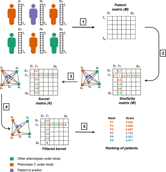
Main logical steps of the P-Net algorithm. For simplicity the graph is shown with n = 6 patients. (1) Each patient is represented by a vector of m features (e.g. expression levels of the genes). Orange patients have the C phenotype; green patients do not show the C phenotype; violet patients are not labelled and our goal is to predict their label. We select the \(m{\prime} < m\) features most correlated with the phenotype C and we use them to construct a \(m{\prime} \times n\) matrix whose n columns represent the bio-molecular profiles of patients restricted to the \({m}^{{\prime} }\) selected features. (2) A W similarity matrix is constructed, where each element wij represents, e.g., the positive filtered Pearson correlation between the patients i and j; note that this matrix can be interpreted as the adjacency matrix of the graph of patients. To make the figure readable we show only the entries of patient p2. (3) The corresponding K kernel matrix is computed through e.g. 2-step Random Walk Kernel. (4) The K matrix is filtered and we remove all the edges with a weight lower than the selected threshold τ = 0.32. (5) A score function (e.g. Nearest Neighbour score) is finally used to compute a score for each patient and to rank them according to their scores.
-
2.
Construction of the patient similarity matrix A matrix W of similarities between biomolecular profiles (full biomolecular profiles or signatures) is obtained from the columns (patients) of M (step 2 of Fig. 1). To construct W we used the filtered Pearson correlation (by setting to zero all negative values), but other measures (e.g. the Spearman correlation or the inverse of some distances, such as the Euclidean or the Manhattan distance) can be used instead. We applied filtered Pearson correlation because other correlation metrics achieved similar or worse results. W can be seen as the adjacency matrix of the weighted graph G, where the edge weights represent the bio-molecular similarity between patients.
-
3.
Computation of a kernel matrix from the patient similarity matrix The kernel matrix K is derived from the similarity matrix W (Fig. 1 - Step 3). This is achieved by choosing a kernel35, able to capture the topological characteristics of the underlying graph. Intuitively, the idea is to derive a new graph where there is an edge between each pair of nodes that is highly connected (i.e. there exist many short paths between them), in the original graph. This means that two nodes may be directly connected in the new graph even if they were not in the original graph (see Fig. 2). Several kernels are suitable for this problem (e.g. the diffusion kernel36), but for our experiments we chose the random walk kernel37,38, since it showed on average better results:
$${\boldsymbol{K}}=(a-1){\boldsymbol{I}}+{{\boldsymbol{D}}}^{-\frac{1}{2}}{\boldsymbol{W}}{{\bf{D}}}^{-\frac{1}{2}}$$where I is the identity matrix, D is the “degree” diagonal matrix with elements dii = ∑jwij and a is a value larger than 2. A p-step random walk kernel can be obtained by simply multiplying K by itself p times. Intuitively, we can think at graph-kernels as functions able to enrich the similarity between nodes in the transformed kernel space, since the novel edge weights of K is determined by the overall topology of the network (e.g. novel edges between vertices are added if a path between them of length equal or less than the steps of the random walk does exist)39. It is worth noting that a graph kernel implicitly induces a new non linear similarity measure between patients, since the novel weights of the computed Gram matrix (i.e. the similarity patient matrix resulting from the application of the kernel) take into account both the topology and the metric distance between the nodes/patients to construct a novel “enriched” similarity graph (Fig. 2).
Figure 2 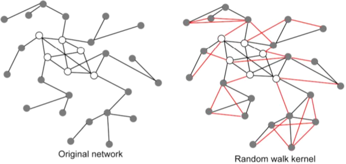
The graph kernel induces a novel similarity measure between patients. The original network (left side of the figure) is constructed using a suitable similarity measure between patients (e.g. the Pearson correlation). The p − step random walk kernel “enriches” the original graph by modifying the weights of the original network and by possibly adding new edges (coloured in red, graph in the right side): if two nodes are indirectly connected through a path of length equal at most to p, a new edge is added between them, and its strength depends on the (possible) multiple paths and the weights of the edges along the paths. In other words the graph kernel implicitly induces a new non linear similarity measure between patients that takes into account the topology of the network and the initial similarity between patients of the original network.
-
4.
Filtering of the kernel matrix The resulting kernel matrix K is usually very dense, and its sparsification is a crucial step that allows to retain only relevant edges, thus reducing the noise introduced by very poor similarities between patients. Unfortunately, simply setting an “a priori” threshold, as usually done in other experimental contexts33,38,39, leads to poor results. To overcome this problem, we select a threshold τ to filter the edges using a very efficient leave-one-out technique that maximizes a pre-selected performance measure (e.g. the Area Under the Receiving Operating Characteristic - AUC) on the training set (see Section “Implementation of P-Net” for more details).
-
5.
Ranking of patients with score functions The score functions associate a score to each node of the network on the basis of the labeling of its neighborhood and the weights of its incoming edges (Table 1). SAV, SNN and SkNN (Eqs. 1, 2 and 3), derived as described in33,34, compute their score respectively considering the average, the nearest and the k nearest labeled neighbours. While these scores exploit only weights coming from the labeled neighbours, the remaining score functions STOT, SDiff and SDnorm (Eqs. 4, 5, and 6) allow us to exploit the information that comes from the whole neighborhood of the investigated node i, including both nodes i ∈ VC and i ∉ VC. In this way the labeling of each node depends on both “positive” and “negative” annotations of the neighborhood nodes.
Table 1 Score functions. Elements of K are represented by kij, and its ith row by Ki, while positive integers i, j represent nodes (patients); VC ⊂ V represents the set of “positive” patients, i.e. patients associated with the phenotype or clinical outcome C of interest.


P-Net provides a score to rank patients, but by setting a threshold τ we can obtain a classifier: patients having a score larger than τ are classified as positive and the others as negative. In our experiments, we set the threshold according to the predicted best accuracy by a fast internal leave-one-out procedure on the training set (see Section “Implementation of P-Net”), and then we applied the selected optimal threshold on the test set. Additional information about P-Net and its implementation are available in the next Section and in the Section “Efficient implementation of P-Net” in the Supplementary Information.
Implementation of P-Net
The analysis of the generalization performances of P-Net and the selection of the network threshold τ (see “Filtering of the kernel matrix” in the “Methods” Section), can be performed through cross-validation or leave-one-out (LOO) procedures. In particular, to obtain an unbiased evaluation of the generalization performance and an unbiased network filtering, we performed a double leave-one-out procedure: (a) an internal LOO to select the network threshold τ; (b) an external LOO to estimate the generalization capabilities of the algorithm.
Unfortunately, the classical implementation of the double LOO requires to run the algorithm n2 times, where n is the number of patients. To avoid this computational burden, we propose an efficient implementation of the P-Net LOO, that requires only a unique run across patients.
Theorem 1: Having a kernel matrix K obtained from the weighted adjacency matrix W of a graph G = <V, E >, with vertices v ∈ V denoted with i ∈ { 1, …, |V|}, and N(i) = {j | j ∈ V, kij > 0} the neighbourhood of node i in the graph G transformed according to the kernel K, when a leave-one-out procedure is applied with the P-Net algorithm, the following fact holds:
Proof:
I. kii = 0 ⇒ node i is left out.
If ∀ i, kii = 0, one of two possible conditions holds:
-
1.
if i ∉ N(i), kii is not included in the computation of the score function S(i), where S is one of the scores functions described in Section “Methods”.
-
2.
if i ∈ N(i), kii is considered in the score function, but by hypothesis kii = 0
In both cases the score of the node i is computed independently of the labeling of the node i, that is, in other words, the node i is left out.
II. kii = 0 ⇐ node i is left out.
If i is left out, even if i ∈ N(i), kii is not used in the computation of the score S. Equivalently we can set kii = 0 and then we can use kii in the computation of S(i), since it has no effect on the computation of the score.□
The intuition behind the efficient LOO implementation is that instead of moving away an example/node at each round of the LOO procedure and recomputing the score for all the nodes of the network, we can equivalently set to zero the self-loop edge of that node. Indeed the information about the labeling of the held-out node i is used only in step 5 of the algorithm (see “Ranking of patients with score functions” in the “P-Net algorithm” section), and by setting kii = 0 we automatically exclude that node by the computation of its score, i.e. we hold-out that node from the training set. As a consequence of the above theorem, to perform the LOO it is sufficient to set to 0 the diagonal of K and then run one time P-Net across all the nodes of the graph G. For instance, to select the optimal threshold τ, we can simply set to zero the diagonal of the kernel matrix K and then apply a unique run of P-Net (Fig. 3).

A P-Net procedure to find the “optimal” filtering threshold τ.
The use of the efficient LOO P-Net procedure for evaluating the generalization performance of the algorithm and to select the optimal threshold of the network are described in detail in the Section “Efficient implementation of P-Net” in the Supplementary Information.
Accession codes
The datasets from Melanoma, Ovarian, Breast, Colorectal and Colon cancer are all available from the Gene Expression Omnibus database (accession numbers GSE53118, GSE26712, GSE2990, GSE17536, GSE17538). The Pancreatic cancer dataset is available from ArrayExpress Archive (accession number E-MEXP-2780).
Results
We compared P-Net with both supervised inductive methods and semi-supervised network-based algorithms for outcome/phenotype prediction. Among supervised inductive methods we selected Support Vector Machines (SVMs) and Random Forests since they showed superior performances for these tasks40,41,42.
We also considered an approach that applies as a first step a network-based method (Net-Rank43), as well as other univariate feature selection methods, to select the most relevant features, and as a second step a supervised algorithm to predict the outcome using the previously selected features26. Net-Rank enhances the Google Pagerank-learning approach44 by using Laplacian regularization and an additive margin: for PageRank the nodes are web pages and the edges are hyperlinks between them; for NetRank the vertices of the network are genes and the edges are relationships between them (e.g. protein-protein or transcription factor-target interactions). Then a Support Vector Machine is trained with the selected features/biomarkers to predict the outcome of patients26.
Finally, we compared our method with an approach developed by Park et al.19. Similarly to P-Net, this method applies a semi-supervised learning algorithm on the similarity graph of patients to rank and classify them according to a specific phenotype/outcome. However this method differs from P-Net since it adopts a solution in closed form to minimize the cost function where both the mislabeling of the patients (the nodes of the graph) and the discrepancy between predicted labels of connected nodes in the graph are jointly minimized. Instead, in our semi-supervised approach, a graph kernel is firstly applied to capture the overall topological characteristics of the graph, and then a score function is applied over the transformed graph to rank patients.
We compared P-Net with each of the above cited methods19,26 by using the same experimental set-up, metrics and datasets used by each of them. We also applied the same filtering approach adopted in the first step of the P-Net algorithm (i.e. a classical t-test) to select the genes significantly associated with the patients’ phenotype/outcome, and we performed gene set enrichment analysis45 to uncover pathways and Gene Ontology terms overrepresented in the set of selected genes, to characterize the underlying disease mechanisms.
The data sets used in the experiments are publicly available and are schematically described in the next section.
Datasets description
We applied our novel P-Net method on several microarray gene expression cancer data sets.
The Pancreatic ductal adenocarcinoma data set from Winter et al.26 includes 30 patients, split into two groups (good prognosis and poor prognosis) according to their survival time (threshold set at 17.5 months, as in the original paper26). The Breast, Colorectal and Colon cancer patients were originally analyzed by Park et al.19. Breast cancer data are composed of 189 invasive breast cancer patients, divided into the classes “high” and “low” risk of recurrence; Colorectal cancer data includes 177 patients and Colon cancer 213, both divided into the groups “recurrence”, “no recurrence”. All these data sets include also “unlabeled” patients, i.e. patients having no prognostic or phenotype associated information. Table 2 shows a high-level summary of the data, and further details are provided in “Datasets” Section of the Supplementary Information.
Analysis of Breast, Colorectal and Colon cancer patients
Experimental set-up
We compared P-Net, using Breast, Colorectal and Colon cancer data, with Park et al. semi-supervised graph-based method that minimizes both the classification error and the “internal consistency” of the predicted labeling19. Moreover we compared P-Net on the same data sets with three other supervised inductive methods, i.e. SVM, Random Forest and Naive Bayes. In the above mentioned experiments we employed the same experimental set-up, based on 10-fold cross-validation, as proposed in19. With these data sets P-Net achieved the best results with a Random Walk Kernel 1-step and the differential or the differential normalized score function (Table 1). More details about the experimental set-up are available in the Section “Experimental set-up for the analysis of Breast, Colorectal and Colon cancer patients” in Supplementary Information.
Results
P-Net outperforms the other methods in terms of the Area Under the Receiving Operating Characteristic (AUROC) (Fig. 4). Moreover the results are statistically significant, according to the one-tail Wilcoxon rank sum test with Bonferroni correction: indeed by applying the statistical test to the repeated 15 cross-validation we always obtain a p-value lower than 0.01 (Table at the bottom of Fig. 4).

Comparison of the average AUROC values obtained by P-Net with the Park’s, Random Forest, Naive Bayes, and SVM methods over three datasets. AUROC results are averaged across 15 rounds of the 10-fold cross-validation. Top: average AUROC with error bars indicating standard deviation (for each dataset, bars are sorted according to decreasing performance). Bottom: statistical comparison of P-Net with the other methods. P-values are computed by one tail Wilcoxon rank sum test across 15 repetitions of 10-fold cross-validation. Rows refer to the methods compared with P-Net; columns to Breast, Colorectal and Colon cancer data.
Also, the accuracy and the sensitivity of P-Net are competitive with the other compared algorithms (see Table S2 Supplementary Information for more details).
Analysis of Pancreatic ductal adenocarcinoma patients
We compared P-Net with a method that applies linear Support Vector Machines trained on biomarkers selected through both a network-based method (NetRank) and other simpler univariate feature selection methods26. We did not use non-linear SVMs since in26 the authors reported that more complex kernels did not lead to better results.
Experimental set-up
Winter et al.26 used NetRank and a series of univariate feature selection methods: fold change, t-statistic, Pearson and Spearman rank correlation coefficients, SAM (Significance Analysis of Microarray) method46, and random selection of genes as control, to select the genes most correlated with the survival time of a patient. Then the selected top ranked genes were used to train a Support Vector Machine (SVM) in order to predict patients with poor (PP) or good (GP) prognosis.
The generalization performances were evaluated through a Monte Carlo cross-validation technique (MCCV). More precisely we randomly split the data in training and test set 1000 times. At each round of the splitting procedure, we performed feature selection through the t-test using only the data of the training set. Then we constructed a network of patients using only the selected genes and we filtered the edges according to the P-Net accuracy on the training set by the efficient leave-one-procedure described in the Section “Implementation of P-Net”. The score threshold to optimally separate poor and good prognosis patients is computed on the training set and the generalization performances are finally evaluated on the separated test. A detailed step by step description of the experimental set-up is available in the Section “Experimental set-up with Pancreatic cancer data” in Supplementary Information.
Results
P-Net used the Random Walk Kernel, and the model with p = 8 steps, the Nearest Neighbour score function and a set of genes selected according to the t-test achieved the best results. Fig. 5 shows the results (average accuracy) for a different number of patients in the training set (from 16 to 28). P-Net achieves better results than the other methods for each training set size, except with 24 patients, where it obtains the second best result. In all cases the difference is statistically significant (t-test at 0.05 significance level). Detailed results showing average accuracy and standard error of the mean for all assessed methods are available in Table 3.

Comparison of the accuracy of P-Net and a SVM trained with NetRank and other feature selection methods on the Pancreatic cancer dataset. P-Net results are shown in red, SVM with NetRank in cyan, the other colors represent the results of the SVM with other feature selection methods (Pearson and Spearman correlation, Fold change, t-test), with random selection and with two other variants of the NetRank algorithm (Direct Neighbour and Constant c). The x axis reports the number of patients in the training set; y axis reports the accuracy.
We performed also an additional experiment to understand whether a larger set of biomarkers selected using a t-test can enhance the performance of the SVM with respect to P-Net. Results show that, even when selecting a relatively large number of biomarkers associated with the poor prognosis (1000 genes), P-Net significantly outperforms the SVM for any size of the training set (Fig. 6).

Comparison of SVM and P-Net after the selection of the top ranked 1000 genes through t-test. The vertical bars represent the Standard Error of the Mean (SEM) of the accuracy across 1000 repetitions of the hold-out procedure.
In the Section “Summary of P-Net results” in the Supplementary Information we report the detailed results obtained by P-Net, including the average AUROC, AUPRC, F1-score and accuracy for each data set. Results show that, as expected, P-Net is more stable when relatively large data sets are used.
Assessment of the statistical significance of the patients ranking
For all the considered data sets, we applied a non parametric test based on random shuffling of the labels to assess the statistical significance of the prediction results47. More precisely we repeat 10000 times a random permutation of the labels, and at each iteration of the shuffling we compare the AUC obtained by P-Net with the “true labels” with that obtained with the randomly permutated labels. The estimated p-value is the frequency by which the AUC computed with the shuffled labels is larger than that computed with the true labels. More details are available in the Section “A non parametric test to validate patient ranking” in the Supplementary Information. Table 4 shows that the computed p-values are always less than 0.05, confirming that the ranking is not due by chance.
Characterization of genes and pathways involved in patients’ outcome
Linking predictions to the underlying disease mechanisms is of paramount importance, and to this end we applied classical gene set enrichment analysis to uncover pathways associated with patients’ phenotype and outcome, starting from the set of genes selected as differentially expressed at the first step of the P-Net algorithm. We excluded from the analysis the pancreatic cancer patients, due to the relatively small number of available examples. More precisely, we selected the genes significantly associated with phenotype/outcome using the classical t-test with Benjamini-Hochberg correction48 at p-value < 0.05 for colorectal and colon cancer and with Bonferroni correction with p-value < 0.001 for breast cancer. The more restrictive Bonferroni correction is needed to obtain a relatively reduced set of differentially expressed genes in breast cancer. We repeated the selection using only genes of the training sets across multiple iterations of the 10-fold cross-validation procedure, and we finally selected only those genes robustly selected at least 70% of times. Each set of robustly selected genes was further analysed using the conditional hypergeometric test to find overrepresented GO:BP terms (p-value < 0.05) and the standard hypergeometric test to discover overrepresented KEGG pathways (p-value < 0.05), as implemented in the R package GOstats45. Since the lists of overrepresented GO terms for breast and colorectal cancer were very large, we used REVIGO49, a clustering algorithm based on semantic similarity measures, to obtain a representative subset of more interpretable terms.
Additionally, the obtained gene lists were analyzed by Ingenuity Pathway Analysis (IPA, QIAGEN Inc., https://www.qiagenbioinformatics.com/products/ingenuity-pathway-analysis) software50 (p-value < 0.05) in order to further investigate enriched signaling and metabolic pathways related to our selected genes.
Results show that we found genes and pathways known to be associated with breast, colon and colorectal cancer, as summarized below. Full lists of the associations, supported by results documented by literature are available in Supplementary Information (Tables S3–S8, Fig. S6).
Breast cancer
364 genes were selected by t-test and used for further functional analysis. Among overrepresented KEGG pathways we found “Proteasome” which is a complex dedicated to protein catabolism involved in several cellular functions (e.g. regulation of cell cycle, signaling pathways, stress signaling, apoptosis). Recent studies suggested that deregulation of the ubiquitin-proteasome pathway may have a permissive role in breast cancer development, and drugs which target this pathway are currently in clinical trial51. From our analysis the pathways “Protein processing in endoplasmic reticulum” and “Oxidative phosphorylation” resulted overrepresented and associated with breast cancer in literature. Endoplasmic reticulum guarantees that only correctly folded proteins reach their final destination in the cell while unfolded/misfolded ones are degraded by the proteasome. However, endoplasmic reticulum stress (ERS), i.e. the accumulation of unfolded/misfolded proteins in the reticulum, may arise due to glucose deficiency, hypoxia, calcium imbalance and oxidative stress. ERS is associated with tumor development and metastasis in breast cancer since the high cell proliferation rate in tumors causes hypoxia, nutrients starvation and higher ROS production52,53. In particular, increased ROS production in cancer cells arises from oxidative phosphorylation, oxygen metabolism and NADPH oxidase functions leading to oxidative stress, described also in breast cancer54.
Considering GO:BP terms, we found some common biological processes known to be involved in tumor development, such as “cell cycle phase transition”, “apoptotic signaling pathway” and “signal transduction by p53 class mediator”. Defects in the cell cycle checkpoints are associated with breast cancer molecular subtypes55 while apoptosis escape is one of the hallmarks of cancer56. p53 is a tumor suppressor able to avoid cancer development through block of the cell cycle, programmed cell death, repair of damaged DNA and senescence. p53 is mutated in 20-30% of breast cancers and it is generally silenced by loss of upstream/downstream mechanisms57. Another interesting term is “cellular oxidant detoxification” which is consistent with the presence of oxidative stress in breast cancer cells58.
Finally, from IPA analysis mTOR-p70S6K signaling resulted enriched in the Top Canonical Pathways, in agreement with its frequent deregulation found in breast cancer, often associated to drug resistance59. The analysis also revealed that “Cell Death and Survival” and “Cellular Growth and Proliferation” are the molecular and cellular functions most significantly overrepresented in the recurrence-associated genes (207 and 139 out of 364 molecules, respectively). These findings are consistent with GO:BP hypergeometric test and the selected genes encoding for cyclins (CCNA2, CCND2), enzymes involved in ubiquitination (UBE2D2, UBE2L3, UBE2N) and the transcription factor STAT1. These results are in line with those obtained by other groups which analyzed GSE2990 dataset60,61,62. In particular, Sotiriou and coworkers reported that genes predicting high risk of recurrence are mainly involved in cell cycle regulation and proliferation60. Of note, STAT1 was identified as a breast cancer recurrence gene also by Park and colleagues62 and it was associated to resistance to endocrine therapy and to distant metastasis-free survival by Huang and others61.
Colon and colorectal cancer
A total of 55 genes were found associated with recurrence in colon and colorectal cancer. In colon cancer, KEGG pathway analysis highlighted dysregulations in few metabolic pathways, such as “Fatty acid biosynthesis”, “Propanoate metabolism” and “Pyruvate metabolism”. Lipid accumulation was observed in many cancer types (e.g. brain, breast, ovarian and colorectal cancers), caused by an imbalance between fatty acid biosynthesis and β-oxidation, where lipids are used by fast growing cells to support various activities like membrane formation and signaling. Abnormal expression of genes involved in fatty acid metabolism was found by different studies in correlation with metastasis, drug resistance and relapse63. Notably, many GO:BP terms found in our analysis are consistent with aberrant lipid metabolism (“malonyl-CoA biosynthetic process”, “negative regulation of fatty acid beta-oxidation”, “carnitine shuttle”, “positive regulation of lipid storage”, “negative regulation of fatty acid metabolic process”, “regulation of fatty acid oxidation”, “acetyl-CoA metabolic process”, “regulation of lipid catabolic process”, “sterol biosynthetic process”, “fatty acid transport”). Considering “Propanoate metabolism” and “Pyruvate metabolism”, most tumor cells highly depend on aerobic glycolysis rather than mitochondrial oxidative phosphorylation to obtain energy, known as “Warburg effect”, and this disregulates the above mentioned metabolic paths64. Moreover, GO:BP analysis revealed multiple terms related to “interleukin mediated signaling pathway” (i.e. IL-2, IL-7, IL-9, IL-12 and IL-15). For instance, Kuniyasu et al.65 associated the production of IL-15 in colon cancer cells with proliferation, resistance to apoptosis, metastasis and angiogenesis.
In colorectal cancer, pathway analysis showed that “Pathogenic Escherichia coli infection” is associated with the disease. Indeed, in literature some strains of E. coli are known to produce a genotoxic metabolite (colibactin) that alkylates DNA in vivo and contributes to the development and progression of this tumor66. Among biological processes consistently overrepresented in our analysis, we found GO:BPs related to the β-catenin destruction complex (i.e. “beta-catenin destruction complex disassembly”, “beta-catenin destruction complex assembly”, “catenin import to nucleus”), nitric-oxide biosynthesis (“positive regulation of nitric oxide biosynthetic process”, “positive regulation of nitric oxide biosynthetic process”, “nitric oxide production involved in inflammatory response”), inflammasome (“positive regulation of NLRP3 inflammasome complex assembly”, “pyroptosis”). The β-catenin destruction complex was recently found disrupted in colorectal cancer67, possibly enabling the migration of β-catenin to the nucleus and the subsequent transcription of target genes. Aberrant stabilization of the β-catenin due to mutations in the destruction complex was associated with various cancers68. Regarding the biosynthesis of nitric-oxide, colorectal cancer is strongly associated with chronic inflammation and nitric-oxide produced by NOS2 is associated with the initiation and progression of the disease. Moreover, over-expression of NOS2 is correlated with poor outcome69. Finally, the activation of NLRP3 inflammasome, with consequent production of IL-1β, IL-18 and procaspase-1 activation which induces pyroptosis (i.e. a form of programmed cell death), showed an anti-tumoral effect preventing/inhibiting colorectal cancer development70.
Functional annotation of selected genes by IPA revealed that 13 out of 54 genes are closely associated to “Cell Growth and Proliferation” and “Cell Death and Survival” (AMER1, ATOH7, CSPP1, CTNNB1, DCD, FGF4, JAK1, NLRC4, PRF1, SLC29A2, SLC4A1, SP7, TRL4). The top canonical pathways enriched for these genes were “Epithelial-Mesenchymal Transition (EMT)”, “Inflammasome” and “iNOS signaling” (see Supplementary Fig. S6). Some pathways were detected by both GOstats and IPA. In particular, EMT pathway has been strongly associated with the invasive and metastatic phenotype in colon cancer71. Among the deregulated genes involved in the EMT signaling, CTNNB1, as well as JAK1 play key roles in colon cancer progression: CTNNB1 through the activation of Wnt/β-catenin signaling, and JAK/STAT pathway by regulating cell survival and proliferation, differentiation and migration72. Our findings are in line with previous studies showing that CTNNB1 and JAK family members are colon cancer recurrence-specific genes and prognostic biomarkers62,72,73,74. Notably, we also identified NLRC4 gene, a member of NOD-like receptors in the “Inflammasome Pathway”, as a novel gene related to colon cancer recurrence. Previous studies have shown that NLRC4 takes part in inflammation-induced colon cancer tumorigenesis and participates in anti-apoptotic pathways downstream of p5375. In addition, a recent study showed that NLRC4 mediates M2 TAM infiltration and angiogenesis through VEGF production in metastatic colon cancer76.
Summarizing, the genes and pathways selected in the first step of P-Net, are not only fundamental to achieve good phenotype/outcome predictions, but are also related to the biological mechanisms underlying the disease.
Visualization of the P-Net graph
Supervised inductive models in most cases are “black boxes” not suitable for interpreting and explaining the obtained results. On the contrary P-Net constructs a graph of patients, explicitly showing their biomolecular relationships and embedding at the same time the predicted scores in the graph. The graph can be easily shown to the user to provide a visual clue of the relationships between patients by means of a graph visualization tool; moreover, the predicted associated phenotype can be properly visualized by exploiting a range of colors and shapes. The user is thus enabled to conduct a direct visual inspection of the network, which might allow him/her to either uncover hidden relationships/insights about the phenotypic and/or biomolecular characteristics of the samples (e.g. disclosing interesting mismatches among similar patients, close in the graph, but with different predicted phenotype), or might suggest stratifications of patients on the basis of their similarity or predicted phenotype.
As an example of this opportunity, Fig. 7 shows the visual representation of the graph constructed by P-Net with the Pancreatic ductal carcinoma data set obtained by adapting to our context a graph visualization tool developed in our laboratory for visualizing biomolecular interactions (the tool is detailed in Perlasca et al.77). In the figure the patient ground truth is shown by the node shapes (circles for good prognosis patients, and rectangles for poor prognosis patients) while the node color shows the prognosis predicted by P-Net. The graphical representation shows that the group of good prognosis patients (highlighted in green) are all correctly predicted by P-Net. A second group (highlighted by a red ellipse) includes poor prognosis patients predicted by our method, some of which are wrongly classified. However, though being labeled as “good prognosis”, the “misclassified patients” are really borderline patients: their survival time is very close to the cut-off of 17.5 months selected in26 to separate good from poor prognosis patients. As another example, Fig. 5 in Supplementary Information visualizes the network of Breast cancer patients.

Pancreatic cancer graph constructed by P-Net. Square nodes represent “poor prognosis”, while circles “good prognosis” patients. The colouring of the nodes is related to the predicted prognosis.
Thus, the graph visualization, eventually coupled with graph clustering algorithms78 and different visualization perspectives and interactions, can allow domain experts to identify interesting visual explanations of the achieved classification, which would not be so evident in a textual representation of the graph. Different approaches have been proposed along this direction, such as77 in the context of biomolecular interactions and79 for the visualization of phenotype similarities. These tools offer different functionalities for clustering graph nodes according to different similarity measures, for changing the color and the shape of the nodes according to different parameters, for changing the layout perspectives and pointing out different graph properties. All these functionalities aid experts to uncover hidden information represented in the graph and to obtain further clues about different patients.
Discussion and Conclusion
P-Net is a semi-supervised transductive approach where the genetic similarities between patients guide the process of outcome prediction and provide a graph representation of the biomolecular similarity between patients. P-Net analyses the biomolecular profiles of patients by firstly constructing a similarity graph between them and then applying a graph kernel, which extends the notion of similarity between patients and exploits the global topology of the graph to discover novel relationships between them. Finally, P-Net ranks patients with respect to the phenotype/outcome under study.
Our experimental results with different cohorts of cancer patients show that this approach is competitive with both network-based and inductive models for outcome prediction. The fast implementation of the P-Net leave-one-out procedure, together with the low spatial and time computational complexity of the method (see Section “Implementation of P-Net” and Supplementary Information), allow an easy application to actual clinical and biomolecular data using off-the-shelf desktop or laptop computers. It is worth noting that by combining different kernels and score functions we can obtain different variants of P-Net. From this standpoint P-Net can be considered as an algorithmic scheme from which specific learning algorithms can be derived by choosing a specific graph kernel and score function.
Several works showed that the outcome results are often not statistically significant and basically due by chance80,81. To address this problem, by using a non parametric test based on random shuffling of the labels, we showed that P-Net ranking of patients is not due by chance, but on the contrary is significantly related to the outcome.
Importantly, P-Net is not only able to predict the phenotype/outcome, but can also construct a graph of patients that can be visualized to point out the similarities between their biomolecular profiles and, more in general, the relationships between them. In this way we can detect, by visual inspection, closely related patients as possible subtypes of a given pathology, or we can identify an incorrect prognosis for a specific patient or for possible “outlier patients”. Finally the filtering step of P-Net can be used not only to improve its prediction performance, but also to link predictions to the underlying disease mechanisms, by uncovering genes and pathways associated with patients’ outcome/phenotype.
It has been shown that the integration of different kinds of data produces synergies between data that can improve the prediction performances82,83,84. To this end we need at first to construct patient similarity networks using similarity measures appropriate for the data at hand. For instance, Pai and Bader for low dimensional data (e.g. clinical data) proposed simple measures such as the normalized and average normalized similarity20. For patient profiles characterized by a medium size, such as mRNA data, protein expression, miRNA, the same authors proposed correlation-based measures (e.g. Spearman, Pearson with and without exponential scaling, euclidean or more in general p-norm distances) with or without an initial pre-filtering (using e.g. univariate statistics or machine learning based feature selection methods). For very high dimensional data (such as genotypic or epigenomic data), a pre-filtering step is mandatory to reduce profiles having a very large number of features. In this context we can adopt a two-steps pre-filtering, e.g. using a fast univariate feature selection method to drop the less significant features and then using a second level multi-variate feature selection method to take into account feature interactions and refine the set of selected features (e.g. classical floating search or branch and bound methods)85. This framework can be integrated with P-Net by substituting its first two steps (data collection and construction of the patient similarity network) with appropriate procedure to construct the network with the different data. Then we have two options to accomplish the integration of the different networks: a) direct integration from the similarity matrices; b) integration after the application of a graph kernel (step 3 of the P-Net algorithm). In both cases we can apply suitable network-based data combination methods, such as simple averaging of the weights of the different networks, or weighted averaging according to the informativeness of each source of data20,29,86 or the SNF methods proposed in83. Considering the large range of possible clinical or omics data that can be used in this context87, and the different similarity measures and integration techniques that can be considered88, we believe that these problems need specific future studies and works that could expand the applicability and the effectiveness of the P-Net learning framework.
A limitation of the proposed approach is that P-Net requires potentially expensive feature selection algorithms to reduce the high dimensionality that usually characterizes genomic data, in order to remove irrelevent features that could add noise to the network of patients. For computational complexity reasons we applied simple univariate methods, but more refined multi-variate methods could lead to better results at the cost of a higher computational time complexity89.
References
Riddick, G. et al. Predicting in vitro drug sensitivity using Random Forests. Bioinformatics 27, 220–224 (2011).
Ruderfer, D. M., Roberts, D. C., Schreiber, S. L., Perlstein, E. O. & Kruglyak, L. Using expression and genotype to predict drug response in yeast. PLoS One 4, e6907 (2009).
Ye, Q.-H. et al. Predicting hepatitis B virus-positive metastatic hepatocellular carcinomas using gene expression profiling and supervised machine learning. Nature Medicine 9, 416–423 (2003).
Chen, Y.-C., Ke, W.-C. & Chiu, H.-W. Risk classification of cancer survival using ANN with gene expression data from multiple laboratories. Computers in Biology and Medicine 48, 1–7 (2014).
Das, J., Gayvert, K. M., Bunea, F., Wegkamp, M. H. & Yu, H. ENCAPP: elastic-net-based prognosis prediction and biomarker discovery for human cancers. BMC Genomics 16, 1 (2015).
Podolsky, M. D. et al. Evaluation of machine learning algorithm utilization for lung cancer classification based on gene expression levels. Asian Pacific Journal of Cancer Prevention 17, 835–838 (2016).
Shipp, M. et al. Diffuse large B-cell lymphoma outcome prediction by gene-expression profiling and supervised machine learning. Nature Medicine 8, 68–74 (2002).
Bartsch, G. et al. Use of artificial intelligence and machine learning algorithms with gene expression profiling to predict recurrent nonmuscle invasive urothelial carcinoma of the bladder. The Journal of Urology 195, 493–498 (2016).
Kim, W. et al. Development of novel breast cancer recurrence prediction model using support vector machine. Journal of Breast Cancer 15, 230–238 (2012).
Kourou, K., Exarchos, T. P., Exarchos, K. P., Karamouzis, M. V. & Fotiadis, D. I. Machine learning applications in cancer prognosis and prediction. Computational and Structural Biotechnology Journal 13, 8–17 (2015).
Guyon, I., Weston, J., Barnhill, S. & Vapnik, V. Gene selection for cancer classification using support vector machines. Machine Learning 46, 389–422 (2002).
Wang, L., Zhu, J. & Zou, H. Hybrid huberized support vector machines for microarray classification and gene selection. Bioinformatics 24, 412–419 (2008).
Colombo, P.-E., Milanezi, F., Weigelt, B. & Reis-Filho, J. S. Microarrays in the 2010s: the contribution of microarray-based gene expression profiling to breast cancer classification, prognostication and prediction. Breast Cancer Research 13, 1 (2011).
Hofree, M., Shen, J., Carter, H., Gross, A. & Ideker, T. Network-based stratification of tumor mutations. Nature Methods 10, 1108–1115 (2013).
Cho, D.-Y. & Przytycka, T. M. Dissecting cancer heterogeneity with a probabilistic genotype-phenotype model. Nucleic Acids Research 41, 8011–8020, https://doi.org/10.1093/nar/gkt577 (2013).
Graim, K. et al. Revealing cancer subtypes with higher-order correlations applied to imaging and omics data. BMC Medical Genomics 10, 20, https://doi.org/10.1186/s12920-017-0256-3 (2017).
Brown, S. A. Patient Similarity: Emerging Concepts in Systems and Precision Medicine. Frontiers in Physiology 7, 561, https://doi.org/10.3389/fphys.2016.00561 (2016).
Kim, Y.-A., Cho, D.-Y. & Przytycka, T. M. Understanding genotype-phenotype effects in cancer via network approaches. PLoS Comput Biol 12, e1004747 (2016).
Park, C., Ahn, J., Kim, H. & Park, S. Integrative gene network construction to analyze cancer recurrence using semi-supervised learning. PLoS One 9, 1–9, https://doi.org/10.1371/journal.pone.0086309 (2014).
Pai, S. et al. netdx: interpretable patient classification using integrated patient similarity networks. Mol. Syst. Biol. 15, e8497, https://doi.org/10.15252/msb.20188497 (2019).
Backstrom, L. & Leskovec, J. Supervised random walks: predicting and recommending links in social networks. In Proceedings of the Forth International Conference on Web Search and Web Data Mining, WSDM 2011, Hong Kong, China, February 9–12, 2011, 635–644, https://doi.org/10.1145/1935826.1935914 (2011).
Zhang, W., Ma, J. & Ideker, T. Classifying tumors by supervised network propagation. Bioinformatics 34, i484–i493, https://doi.org/10.1093/bioinformatics/bty247 (2018).
Barabási, A. L., Gulbahce, N. & Loscalzo, J. Network medicine: a network-based approach to human disease. Nature Reviews Genetics 12, 56–68 (2011).
Moreau, Y. & Tranchevent, L.-C. Computational tools for prioritizing candidate genes: boosting disease gene discovery. Nature Reviews Genetics 13, 523–536 (2012).
Lippert, G., Ghahramani, Z. & Borgwardt, K. Gene function prediction from synthetic lethality networks via ranking on demand. Bioinformatics 26, 912–918 (2010).
Winter, C. et al. Google Goes Cancer: Improving Outcome Prediction for Cancer Patients by Network-Based Ranking of Marker Genes. PLoS Computational Biology 8 (2012).
Kohler, S., Bauer, S., Horn, D. & Robinson, P. Walking the interactome for prioritization of candidate disease genes. Am. J. Human Genetics 82, 948–958 (2008).
Ideker, T. & Krogan, N. J. Differential network biology. Molecular Systems Biology 8, 565 (2012).
Valentini, G., Paccanaro, A., Caniza, H., Romero, A. E. & Re, M. An extensive analysis of disease-gene associations using network integration and fast kernel-based gene prioritization methods. Artificial Intelligence in Medicine 61, 63–78 (2014).
Nguyen, T.-P. & Ho, T.-B. Detecting disease genes based on semi-supervised learning and protein-protein interaction networks. Artificial Intelligence in Medicine 54, 63–71 (2012).
Navarro, C., Martínez, V., Blanco, A. & Cano, C. Prophtools: general prioritization tools for heterogeneous biological networks. GigaScience 6, 1–8, https://doi.org/10.1093/gigascience/gix111 (2017).
Le Morvan, M., Zinovyev, A. & Vert, J.-P. Netnorm: Capturing cancer-relevant information in somatic exome mutation data with gene networks for cancer stratification and prognosis. PLoS Computational Biology 13, e1005573, https://doi.org/10.1371/journal.pcbi.1005573 (2017).
Re, M. & Valentini, G. Cancer module genes ranking using kernelized score functions. BMC Bioinformatics 13, https://doi.org/10.1186/1471-2105-13-S14-S3 (2012).
Valentini, G. et al. RANKS: a flexible tool for node label ranking and classification in biological networks. Bioinformatics 32, 2872–2874, https://doi.org/10.1093/bioinformatics/btw235 (2016).
Shawe-Taylor, J. & Cristianini, N. Kernel Methods for Pattern Analysis (Cambridge University Press, Cambridge, UK, 2004).
Picart-Armada, S., Thompson, W., Buil, A. & Perera-Lluna, A. “diffustats: an r package to compute diffusion-based scores on biological networks”. Bioinformatics, btx632, https://doi.org/10.1093/bioinformatics/btx632 (2017).
Smola, A. J. & Kondor, R. Kernels and regularization on graphs. In Schölkopf, B. and Warmuth, M. K. (eds) Learning Theory and Kernel Machines: 16th Annual Conference on Learning Theory and 7th Kernel Workshop, COLT/Kernel 2003, Washington, DC, USA, August 24–27, 2003. Proceedings, 144–158 (Springer Berlin Heidelberg, Berlin, Heidelberg, 2003).
Re, M., Mesiti, M. & Valentini, G. A Fast Ranking Algorithm for Predicting Gene Functions in Biomolecular Networks. IEEE ACM Transactions on Computational Biology and Bioinformatics 9, 1812–1818 (2012).
Re, M. & Valentini, G. Network-based Drug Ranking and Repositioning with respect to DrugBank Therapeutic Categories. IEEE/ACM Transactions on Computational Biology and Bioinformatics 10, 1359–1371 (2013).
Barter, R. L., Schramm, S.-J., Mann, G. J. & Yang, Y. H. Network-based biomarkers enhance classical approaches to prognostic gene expression signatures. BMC Systems Biology 8, S5, https://doi.org/10.1186/1752-0509-8-S4-S5 (2014).
Statnikov, A., Wang, L. & Aliferis, C. A comprehensive comparison of random forests and support vector machines for microarray-based cancer classification. BMC Bioinformatics 9, 319, https://doi.org/10.1186/1471-2105-9-319 (2008).
Chen, X. & Ishwaran, H. Random forests for genomic data analysis. Genomics 99, 323–329, https://doi.org/10.1016/j.ygeno.2012.04.003 (2012).
Agarwal, A. & Chakrabarti, S. Learning random walks to rank nodes in graphs. In Proceedings of the 24th International Conference on Machine Learning, ICML ’07, 9–16, https://doi.org/10.1145/1273496.1273498 (ACM, New York, NY, USA, 2007).
Page, L., Brin, S., Motwani, R. & Winograd, T. Page, L., Brin, S., Motwani, R. and Winograd, T. The pagerank citation ranking: Bringing order to the web. Tech. Rep., Stanford InfoLab (1999).
Falcon, S. & Falcon, S. Using GOstats to test gene lists for GO term association. Bioinformatics 23, 257–258, https://doi.org/10.1093/bioinformatics/btl567, http://oup.prod.sis.lan/bioinformatics/article-pdf/23/2/257/532391/btl567.pdf (2006).
Tusher, V., Tibshirani, R. & Chu, G. Significance analysis of microarrays applied to the ionizing radiation response. Proceedings of the National Academy of Sciences 98, 5116–5121, https://doi.org/10.1073/pnas.091062498, http://www.pnas.org/content/98/9/5116.full.pdf (2001).
Edgington, E. & Onghena, P. Randomization tests (Chapman and Hall, New York, 2007).
Benjamini, Y. & Hochberg, Y. Controlling the false discovery rate: A practical and powerful approach to multiple testing. Journal of the Royal Statistical Society. Series B (Methodological) 57, 289–300 (1995).
Supek, F., Bošnjak, M., Škunca, N. & Šmuc, T. Revigo summarizes and visualizes long lists of gene ontology terms. PLoS One 6, 1–9, https://doi.org/10.1371/journal.pone.0021800 (2011).
Krämer, A., Green, J., Pollard, J. Jr. & Tugendreich, S. Causal analysis approaches in Ingenuity Pathway Analysis. Bioinformatics 30, 523–530, https://doi.org/10.1093/bioinformatics/btt703, http://oup.prod.sis.lan/bioinformatics/article-pdf/30/4/523/17343942/btt703.pdf (2013).
Cardoso, F., Ross, J. S., Piccart, M. J., Sotiriou, C. & Durbecq, V. Targeting the ubiquitin-Ťproteasome pathway in breast cancer. Clinical Breast Cancer 5, 148–157, https://doi.org/10.3816/CBC.2004.n.020 (2004).
Han, C.-c & Wan, F.-S. New insights into the role of endoplasmic reticulum stress in breast cancer metastasis. Journal of breast cancer 21, 354–362 (2018).
Sisinni, L. et al. Endoplasmic reticulum stress and unfolded protein response in breast cancer: The balance between apoptosis and autophagy and its role in drug resistance. International Journal of Molecular Sciences 20, https://doi.org/10.3390/ijms20040857 (2019).
Mencalha, A., Victorino, V. J., Cecchini, R. & Panis, C. Mapping oxidative changes in breast cancer: understanding the basic to reach the clinics. Anticancer research 34, 1127–1140 (2014).
Bower, J. J. et al. Patterns of cell cycle checkpoint deregulation associated with intrinsic molecular subtypes of human breast cancer cells. NPJ Breast Cancer 3, 9 (2017).
Plati, J., Bucur, O. & Khosravi-Far, R. Dysregulation of apoptotic signaling in cancer: Molecular mechanisms and therapeutic opportunities. Journal of Cellular Biochemistry 104, 1124–1149 (2008).
Moulder, D. E., Hatoum, D., Tay, E., Lin, Y. & McGowan, E. M. The roles of p53 in mitochondrial dynamics and cancer metabolism: The pendulum between survival and death in breast cancer? Cancers 10, https://doi.org/10.3390/cancers10060189 (2018).
Nourazarian, A. R., Kangari, P. & Salmaninejad, A. Roles of oxidative stress in the development and progression of breast cancer. Asian Pac J Cancer Prev 15, 4745–51 (2014).
Hare, S. H. & Harvey, A. J. mtor function and therapeutic targeting in breast cancer. Am. journal of cancer research 7, 383 (2017).
Sotiriou, C. et al. Gene Expression Profiling in Breast Cancer: Understanding the Molecular Basis of Histologic Grade To Improve Prognosis. JNCI: Journal of the National Cancer Institute 98, 262–272, https://doi.org/10.1093/jnci/djj052, http://oup.prod.sis.lan/jnci/article-pdf/98/4/262/7688280/djj052.pdf (2006).
Huang, R. et al. Increased stat1 signaling in endocrine-resistant breast cancer. PLoS One 9, 1–11, https://doi.org/10.1371/journal.pone.0094226 (2014).
Park, C., Ahn, J., Kim, H. & Park, S. Integrative gene network construction to analyze cancer recurrence using semi-supervised learning. PLoS One 9, e86309 (2014).
Kuo, C.-Y. & Ann, D. K. When fats commit crimes: fatty acid metabolism, cancer stemness and therapeutic resistance. Cancer Communications 38, 47 (2018).
Fan, T. et al. Tumor energy metabolism and potential of 3-bromopyruvate as an inhibitor of aerobic glycolysis: implications in tumor treatment. Cancers 11, 317 (2019).
Kuniyasu, H. et al. Production of interleukin 15 by human colon cancer cells is associated with induction of mucosal hyperplasia, angiogenesis, and metastasis. Clinical Cancer Research 9, 4802–4810, https://clincancerres.aacrjournals.org/content/9/13/4802.full.pdf (2003).
Wilson, M. R. et al. The human gut bacterial genotoxin colibactin alkylates dna. Science 363, https://doi.org/10.1126/science.aar7785, https://science.sciencemag.org/content/363/6428/eaar7785.full.pdf (2019).
Bourroul, G. M. et al. The destruction complex of beta-catenin in colorectal carcinoma and colonic adenoma. Einstein (São Paulo) 14, 135–142 (2016).
Stamos, J. L. & Weis, W. I. The β-catenin destruction complex. Cold Spring Harbor perspectives in biology 5, a007898 (2013).
de Oliveira, G. A. et al. Inducible nitric oxide synthase in the carcinogenesis of gastrointestinal cancers. Antioxidants & Redox Signaling 26, 1059–1077, https://doi.org/10.1089/ars.2016.6850, PMID: 27494631 (2017).
Moossavi, M., Parsamanesh, N., Bahrami, A., Atkin, S. L. & Sahebkar, A. Role of the nlrp3 inflammasome in cancer. Molecular cancer 17, 158 (2018).
Vu, T. & Datta, P. K. Regulation of emt in colorectal cancer: A culprit in metastasis. Cancers 9, https://doi.org/10.3390/cancers9120171 (2017).
Tang, S. et al. Association analyses of the jak/stat signaling pathway with the progression and prognosis of colon cancer. Oncology letters 17, 159–164 (2019).
Chen, Y. & Song, W. Wnt/catenin β 1/microrna 183 predicts recurrence and prognosis of patients with colorectal cancer. Oncology letters 15, 4451–4456 (2018).
Yoshida, N. et al. Analysis of wnt and β-catenin expression in advanced colorectal cancer. Anticancer research 35, 4403–4410 (2015).
Hu, B. et al. Inflammation-induced tumorigenesis in the colon is regulated by caspase-1 and nlrc4. Proceedings of the National Academy of Sciences 107, 21635–21640 (2010).
Ohashi, K. et al. Nod-like receptor c4 inflammasome regulates the growth of colon cancer liver metastasis in nafld. Hepatology (2019).
Perlasca, P. et al. Unipred-web: a web tool for the integration and visualization of biomolecular networks for protein function prediction. BMC Bioinform. 20, https://doi.org/10.1186/s12859-019-2959-2 (2019).
Schaeffer, S. E. Survey: Graph clustering. Comput. Sci. Rev. 1, 27–64, https://doi.org/10.1016/j.cosrev.2007.05.001 (2007).
Peng, J. et al. An online tool for measuring and visualizing phenotype similarities using hpo. BMC Genomics 19, 571, https://doi.org/10.1186/s12864-018-4927-z (2018).
Venet, D., Dumont, J. E. & Detours, V. Most random gene expression signatures are significantly associated with breast cancer outcome. PLoS Comput Biol 7, e1002240 (2011).
Michiels, S., Koscielny, S. & Hill, C. Prediction of cancer outcome with microarrays: a multiple random validation strategy. The Lancet 365, 488–492 (2005).
Cesa-Bianchi, N., Re, M. & Valentini, G. Synergy of multi-label hierarchical ensembles, data fusion, and cost-sensitive methods for gene functional inference. Machine Learning 88, 209–241 (2012).
Wang, B. et al. Similarity network fusion for aggregating data types on a genomic scale. Nature methods 11, 333–337 (2014).
Caceres, J. & Paccanaro, A. Disease gene prediction for molecularly uncharacterized diseases. PLoS Comput Biol 15, e1007078, https://doi.org/10.1371/journal.pcbi.1007078 (2019).
Somol, P., Pudil, P. & Kittler, J. Fast branch and bound algorithms for optimal feature selection. IEEE Transactions on Pattern Analysis and Machine Intelligence 26, 900–912 (2004).
Bersanelli, M. et al. Methods for the integration of multi-omics data: mathematical aspects. BMC Bioinformatics 17, S15, https://doi.org/10.1186/s12859-015-0857-9 (2016).
Pai, S. & Bader, G. Patient Similarity Networks for Precision Medicine. Journal of Molecular Biology 430, 2924–2938, https://doi.org/10.1016/j.jmb.2018.05.037 (2018).
Caniza, H., Romero, A. & Paccanaro, A. A network medicine approach to quantify distance between hereditary disease modules on the interactome. Scientific Reports 5, 17658 (2015).
Wang, L., Wang, Y. & Chang, Q. Feature selection methods for big data bioinformatics: A survey from the search perspective. Methods 111, 21–31, https://doi.org/10.1016/j.ymeth.2016.08.014, Big Data Bioinformatics (2016).
Acknowledgements
A.PA. is supported by Biotechnology and Biological Sciences Research Council (https://bbsrc.ukri.org/) grants BB/K004131/1, BB/F00964X/1 and BB/M025047/1, Consejo Nacional de Ciencia y Tecnología Paraguay - CONACyT (http://www.conacyt.gov.py/) grants 14-INV-088 and PINV15-315, and National Science Foundation Advances in Bio Informatics (https://www.nsf.gov/) grant 1660648; G.V. is supported by “Fondo per il finanziamento delle attività base di ricerca” funded by Ministero dell’Istruzione dell’Università e della Ricerca (http://www.miur.gov.it/), grant 25537; M.M. and P.P. are supported by “Ministero dell’Istruzione dell’Università e della Ricerca (http://www.miur.gov.it/) - Annual Financial Support for Research – FFABR2018_DIP_010_MESITI”; E.C. and G.G. are supported by “Bando Sostegno alla Ricerca, LINEA A - Università degli Studi di Milano (http://www.unimi.it/) Project Title: Nuclei segmentation from histological images“. The funders had no role in study design, data collection and analysis, decision to publish, or preparation of the manuscript.
Author information
Authors and Affiliations
Contributions
All the authors contributed to this paper. Conceptualization and methodology: J.G., G.V., A.PA and M.R. Project administration: G.V., A.PA. Formal analysis: G.V., M.M., M.F., M.R. and G.G. Data Curation and Investigation: J.G., M.M., P.P., E.C., M.R., G.G., V.V., E.V. Software: J.G., G.V. Supervision: A.PA and G.V. Validation: J.G., P.P. and M.M. Visualization: P.P., M.M., J.G. Funding acquisition: M.M., P.P., G.G., A.PA, M.R., G.V. Writing - Original Draft Preparation: J.G., G.V. and A.PA. Writing - Review & Editing: all the authors.
Corresponding authors
Ethics declarations
Competing interests
The authors declare no competing interests.
Additional information
Publisher’s note Springer Nature remains neutral with regard to jurisdictional claims in published maps and institutional affiliations.
Supplementary information
Rights and permissions
Open Access This article is licensed under a Creative Commons Attribution 4.0 International License, which permits use, sharing, adaptation, distribution and reproduction in any medium or format, as long as you give appropriate credit to the original author(s) and the source, provide a link to the Creative Commons license, and indicate if changes were made. The images or other third party material in this article are included in the article’s Creative Commons license, unless indicated otherwise in a credit line to the material. If material is not included in the article’s Creative Commons license and your intended use is not permitted by statutory regulation or exceeds the permitted use, you will need to obtain permission directly from the copyright holder. To view a copy of this license, visit http://creativecommons.org/licenses/by/4.0/.
About this article

Cite this article
Gliozzo, J., Perlasca, P., Mesiti, M. et al. Network modeling of patients' biomolecular profiles for clinical phenotype/outcome prediction. Sci Rep 10, 3612 (2020). https://doi.org/10.1038/s41598-020-60235-8
Received:
Accepted:
Published:
DOI: https://doi.org/10.1038/s41598-020-60235-8
This article is cited by
-
Exploring the similarity between genetic diseases improves their differential diagnosis and the understanding of their etiology
European Journal of Human Genetics (2024)
-
LanDis: the disease landscape explorer
European Journal of Human Genetics (2024)
Comments
By submitting a comment you agree to abide by our Terms and Community Guidelines. If you find something abusive or that does not comply with our terms or guidelines please flag it as inappropriate.
